[Fang+:PACT05] Instruction Based Memory Distance Analysis and its Application to Optimization

In this paper, Fang et. al. extended the notion of memory distance, e.g. reuse distances, to applying on the instruction space of a program, guiding feedback-directed optimization. Memory distance is a dynamic quantifiable distance in terms of memory references between two accesses to the same memory location. The use of memory distance is to predict the miss rates of instructions in a program. Using the miss rates, the author then identified the program’s critical instructions – the set of high miss instructions whose cumulative misses account for 95% of the L2 cache misses in the program – in both integer and floating-point programs. In addition, memory distance analysis is applied to memory disambiguation in out-of-order issue processors, using those distances to determine when a load may be speculated ahead of a preceding store.

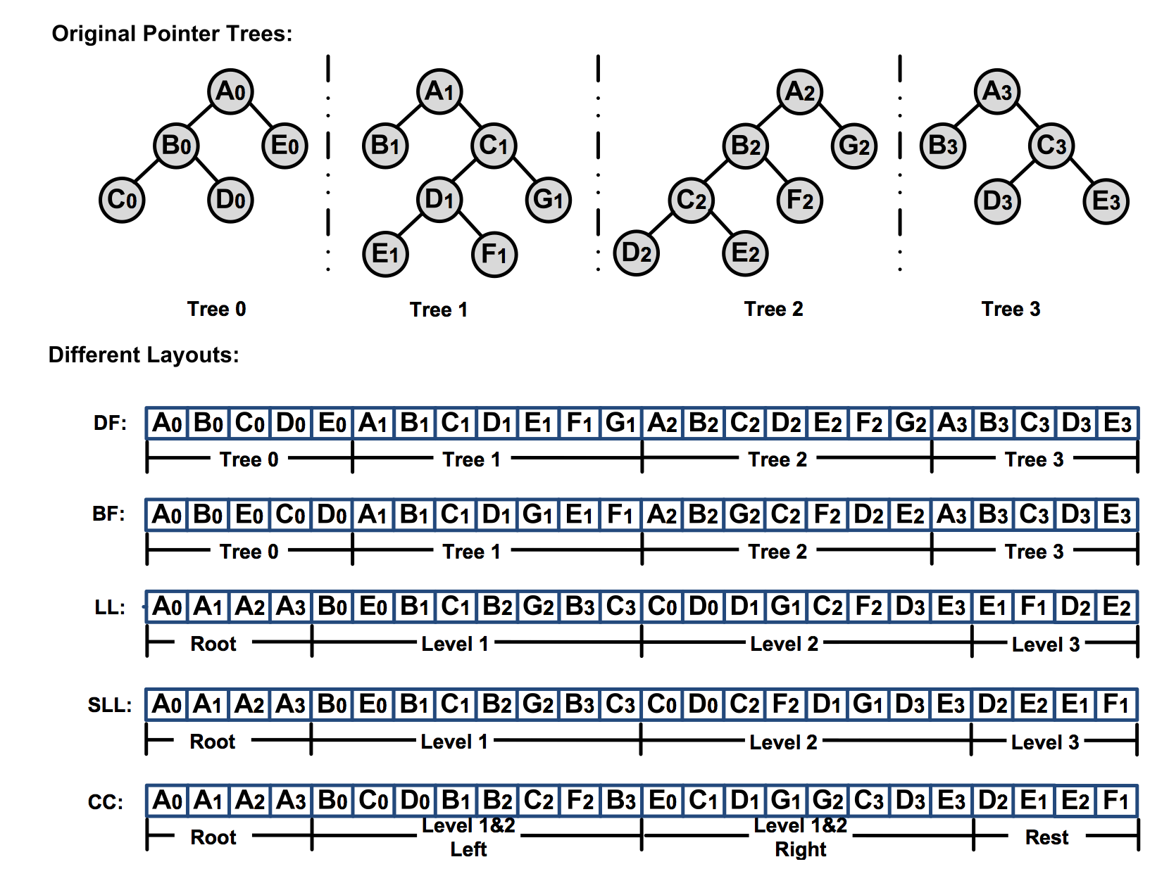
The authors define the notion of memory distance as any dynamic quantifiable distance in terms of memory references between two accesses to the same memory location. Reuse distance is thus a special case of memory distance. The contribution of the work is an algorithm to predict the reuse distance distribution and miss rate for each instruction. The major overhead is storage. For each instruction, a series of log-scale bins is maintained, each bin is attributed by min, max, mean, frequency (access count). The bins is the full reuse distance representation of an instruction. Adjacent bins can be merged to form a locality pattern .The locality pattern is approximated by a linear distribution of reuse distances. The locality patterns is

a compact representation of reuse distances. In order to use the training run’s reuse distance profiles to predict other run’s reuse distance, the authors also define the prediction coverage, (whether the instruction is present in test run if it was in training run) and prediction accuracy (whether the reuse distances in training runs are roughly match the reuse distances in test runs). The authors found that linearly merging bins into patterns improves the prediction accuracy.

Using reuse distances to predict miss rate is very straightforward. No conflict misses are modeled. Using per-instruction reuse distances to identify critical instructions is also easy to do. The authors found that critical instructions tend to have more diverse locality patterns than non-critical instructions. Critical instructions also tend to exhibit a higher percentage of non-constant patterns than non-critical instructions.

The authors introduce two new forms of memory distance – access distance and value distance – and explore the potential of using them to determine which loads in a program may be speculated. The access distance of a memory reference is the number of memory instructions between a store to and a load from the same address. The value distance of a reference is defined as the access distance of a load to the first store in a sequence of stores of the same value.

The intuition is for speculative execution, if a load is sufficiently far away from the previous store to the same address, the load will be a good speculative candidate. Access distance can be used to model this notion for speculation. When multiple successive stores to the same address write the same value, a subsequent load to that address may be safely moved prior to all of those stores except the first as long as the memory order violation detection hardware examines the values of loads and stores. Value distance can be used to model this effect.

[Mohammad+:ASPLOS13]Traffic Management: A Holistic Approach to Memory Placement on NUMA Systems

Better utilization on cache usually results in better performance, but this paper shows in NUMA architecture, memory accesses balance is more important than locality on local LLC.

NUMA

NUMA machines are consist by more than 2 sockets, each of them has independent memory controller and cache. Form a socket’s perspective, its own cache/memory are defined as local cache/memory, and others are remote ones. Sockets transform data through interconnection bus. They access data with following rules:

1.If datum is not in local cache, turns 2

2.Require datum from remote cache, if there is no datum in that cache, turns 3

*3.read data from remote memory

The architecture and overheads are showed with followed figure.

From "Traffic Management: A Holistic Approach to Memory Placement on NUMA Systems"

From “Traffic Management: A Holistic Approach to Memory Placement on NUMA Systems”

Issues

Remote access latency has a higher overhead, thus an intuitively thinking is higher local cache access ratio will result in better performance. But in this paper author found that, when serious congestion comes up, latency of accessing remote memory will incredibly  increasing, says from 300 to 1200 cycles.

They show this issues by firstly show the overhead of congestion, by comparing two different memory placement scenario. The first one is First touch scenario(F), “the default policy where the memory pages are placed on the node where they are first accessed”. The second one is Interleaving (I) – “where memory pages are spread evenly across all nodes.” These two scenarios are showed in Fig 3 of that paper. It is obviously that F has better cache

With experiments on NAS, PARSEC and map/reduce Metis suits, authors shows that in 9 of 20 benchmarks, F is the better one and only in 5 benchmarks, I is better. Which is also showed in Fig 2(b). But, in 3 programs, I gets more than 35% better performance than F. In other side, all of F get not more than 30% better performance than I except one.

And then they showed two cases study in Table 1 that , even some program has better local access ratio(25% vs 32%), but its higher memory latency(465 vs 660) also regrades the performance.

Approach

They use four strategies to reduce congestion and improve locality:

1.Page relocation : “when we re-locate the physical page to the same node as the thread that accesses it”

2.Page replication: “placing a copy of a page on several memory nodes”

3.Page interleaving : “evenly distributing physical pages across nodes.”

*4.Thread clustering : “co-locating threads that share data on the same node”

The workflow is showed in followed figure:

From "Traffic Management: A Holistic Approach to Memory Placement on NUMA Systems"

From “Traffic Management: A Holistic Approach to Memory Placement on NUMA Systems”

[Denning’76]Properties of the Working-Set Model

The Working-Set models motivates to design adaptive memory management policies based on analytic program behaviors. A program’s working set is the smallest subset of its pages that have to reside in memory provided the program operates at a desired level of efficiency.

Consider a program with n pages, constituting the set N = 1, 2, . . . , n, the reference string is a sequence of pages, i.e. p = r1r2 …rt …, each rt being in N. rt = i denotes page i is referenced at the t-th reference. A locality is a subset of its mostly recent referenced pages. A reference missing of page is defined as a referenced page is not in the locality set. A locality set is a working-set.

Next let’s define working set, missing-page rate and inter-reference interval precisely.

A Working-set W(t,T) is the set at time t of distinct pages referenced in the time range [t − T + 1, t]. T is window size. Then we can compute the average number of distinct pages of some window size T.

s(T) = \lim_{k\rightarrow \infty} \frac{1}{k}\sum_{t=1}^{k}w(t,T)

where w(t,T) is the size of W(t,T) set.

The missing-page rate m(T) measures the number of page references per unit time not in the working set. ∆(t,T) = 1 if rt+1 is not in W(t,T), 0 otherwise.

m(T) = \lim_{k\rightarrow \infty} \frac{1}{k}\sum_{t=0}^{k-1}\Delta (t,T)

In a reference string r1r2 . . . rt . . ., two successive references to pages i occur at times t and t + xi, we call xi an inter-reference interval for page i. The inter-reference interval distribution of page i is defined as

F_i(x) = \lim_{k\rightarrow \infty} \frac{{\textit{no. }}x_i \in r_1\dots r_k \textit{ with } x_i \le x}{\textit{ no. }x_i \in r_1\dots r_k }

Based on three assumptions related with locality, 1) reference strings are endless, 2) the stochastic mechanism underlying the generation of a reference string is stationary, and 3) references are asymptotically uncorrelated, the working-set theory has the relationships among average working- set size, missing-page rate and the inter-reference-interval distribution can be derived from both time-average statistics and window-average statistics.

[Wang+:CGO’10]On Improving Heap Memory Layout by Dynamic Pool Allocation

Dynamic memory allocation could occupies a large portion of program running time[Detlefs et al.94]. General-purpose memory allocators often concentrate more on balance between perfor- mance and memory space utilization. They put less attention on specific characteristics of memory allocated heap objects, say the data structures of heap objects.

Pool allocation is a technique that aggregates heap objects at the time of their allocation into separate pools according to types of heap objects, say lists, trees, graph nodes. Doing so, a better data locality can be accomplished, since programs always traverse the same type of objects at the same time. Lattner et al.[Lattner et al.PLDI05] uses compile-time analysis to achieve pool allocation to improve cache locality. The effect is good due to cache miss reductions, and TLB miss reductions meanwhile for the same reason as cache.

However, static analysis is not reliable all the time and in some cases source programs are not available for analysis. Hence, this work comes up with a lightweight dynamic pool allocation tool(DPA), which aggregates the objects which have affinity together at run-time to change heap layout.

The key of dynamic pool allocation is to determine which object goes to which memory pool. At run-time, without source-code level information, it is hard to decide data structures of objects. One existing work is called call-site based strategy[Zhao et al.05]. The objects allocated at the same call-site have the same types.

However, there are two challenges for this strategy. The first is caused by the wrapper functions used by users to safe-guard built-in malloc, which is frequently used by today’s programmers. That being said, in this case the distinct types of objects are considered as the same type because of the same call-site. The second challenge is that heap objects of a data structure could be allocated through different call-sites.

To solve the first challenge, the paper uses a method called adaptive partial call chain to decide a more reasonable call-site for an allocation. It uses stack unwinding to trace back the call stack in order to know calling context information of current procedure. By cutting partial call chain of memory allocation function, it gets the so-called call-site for a malloc.

To solve the second challenge, object group merging approach is proposed. An object group is defined as a set of objects which are put in the same memory pool. By merging object groups with the same affinity, eventually the work figures out the minimum number of object groups, i.e. the minimum number of memory pools. The paper defines two affinities. Objects are of type-1 affinity if they are of the same data type and are linked to form a data structure, say a list, a tree and a graph. The objects are of type-2 affinity if they are pointed by the member fields of type-1 objects and are of the same data structure. All objects and object groups that are of the same affinity can be merged.

After object groups are found, the work allocates a continuous amount of memory space for a memory pool. The work evaluated DPA on several SPEC CPU2000 and 2006 benchmark programs that use extensive heap objects. Results show it could achieve average speedups of 12.1% and 10.8% on two x86 machines in contrast to GCC -O3.

[Shen+:EXPCS07] Analysis of Input-Dependent Program Behavior Using Active Profiling

Introduction

————

Profiling repetitive behavior in programs has historically been difficult. “Active profiling” identifies program phases by controlling the input of the program, and monitoring the occurrences of basic blocks in execution.

There are two important definitions:

(1) Phase: “A unit of predictable behavior in that its instances, each of which is a continuous segment of program execution, are similar in some important respect.”

(2) Phase Marker: A basic block that, when executed, is always followed by an instance of the program phase it marks.

Screen Shot 2015-03-18 at 9.54.06 AM

The above figure (Figure 2 in the paper) shows the IPC over logical time for GCC compiling a series of identical loops.

Selecting Phase Markers
———————–

The paper presents a 3-step method for identifying phase markers:

(1) The program is given a test input with f identical requests (e.g. in the figure compiling the same loop f times). Basic blocks which execute exactly f times are then selected as potential phase markers. Candidate phase markers whose inter-occurrence distances vary significantly are removed from consideration (because actual phase markers should occur at regular intervals).

(2) Analysis tests whether each remaining candidate occurs g times with other inputs that have g non-identical requests. If not, the candidate is removed from consideration.

(3) In step 3, inner-phases and their phase markers are identified.

Evaluation
———-

They test their system on 3 different programs with repetitive inputs, and show figures with phase markers for each:

(1) GCC: 4 identical functions.

(2) Compress: “A file that is 1% of the size of the reference input in the benchmark suite”. Compress has inherent repetition, because it compresses and decompresses the same input 25 times.

(3) L1: 6 Identical Expressions.

(4) Parser: 6 copies of a difficult-to-parse sentence.

(5) Vortex: A database and 3 iterations of lookups.

Uses of Behavior Phases
———————–

Garbage Collection: A behavior phase “often represents a memory usage cycle, in which temporary data are allocated in early parts of a phase and are dead by the end of the phase”. If garbage collection is run at the end of the phase, there is likely to be a higher fraction of garbage. Shen et al. implemented “preventive” garbage collection and applied it to the Lisp interpreter L1. (The standard “reactive” type of GC collects when the heap is full). Their testing results showed that preventive GC can result in faster execution times than reactive GC. However, in the test they showed, not using GC was faster than either of the GC options, so I’m not sure what to make of their result.

Memory Leak Detection: “If a site allocates only phase-local objects during profiling, and if not all its objects are freed at the end a phase, it is likely that the remaining objects are memory leaks.” This observation can be used to give programmers recourse to find memory leaks. Additionally, phase-local objects that are not freed by the end of the phase can be placed on the same virtual memory page. If not used, they will just go to disk, and not clog up memory.

[zhou+:NPC14] An Ecient Simulation Algorithm for Cache of Random Replacement Policy

Shuchang Zhou proposed a efficient algorithm to calculating the hit probability for cache with random replacement policy.

How much one cache can influence performance are often evaluated by running a cache simulator by collected traces. Different associativities, sizes and replacement policies will lead to different result. But for one special cache with random replacement policies, single round simulation can only gives one possible result of performance because of the randomness. So we have to run the simulation multiple times to get a average performance which is very inefficiency.

Based on this observation, they came up with a efficient way to calculate hit probability of each memory access by using expectation, which can be used to derive miss ratio.

Foundation:

      The trace of the accessed sequence (cache lines) is:

               a0, a1, a2, …, aN.

     The miss event of time i is Xi. if a miss event happens at i, then Xi = 1, else Xi = 0.

               X0, X1, X2, … XN.

      So the hit event will be 1-Xi at time i.


       Assume k is the time when the reuse window starts, the number of misses since k to time i will be Zi.

            If the reuse window exists,

                    Zi = sum(Xl), ( k+1<=l<= i-1 )

             Else,

                     Zi = infinite

      The expectation will be the following according to the linearity of expectation,

                     E(Zi) = sum( E(Xl) ) , ( k+1<=l<= i-1 ) or infinite


        With the definition number of misses Zi, E(Xi) can be defined as:

                       E(Xi) = 1 – E( (1-1/M)^Zi ), M is the cache size

         When M is very large,

                       E(Xi) ~ 1-(1-1/M)^E(Zi)

         Proof:

                        if Zi == infinite:

                                 1-(1-1/M)^E(Zi) = 1 – E( (1-1/M)^Zi ) = 0

                         Else:

                                  1.001

      Then they proposed two algorithms to calculate E(Zi ) efficiently from E(Xi) and compared the results with average 5, 50, 500 round naive simulation which proves their method has less error.

Efficient Computation of Reuse Distance

Characterizing the memory performance of today’s diverse workloads is an important and challenging problem. Considering their bursty, irregular, and dynamic behavior along with limited available resource, achieving efficient and accurate characterization has been the focus of many research papers in the field.

Denning’s working set theory lead to the first abstraction for memory performance. Simply, extract the phases of a program and then compute the working set size of each program. With the development of caching memories, choosing the cache size became an important performance decision. This choice required a method that can approximate the program’s memory performance under different cache sizes; the miss ratio curve. However, at the time, the best practice for computing such a curve was Mattson’s original stack simulation algorithm, which required O(MN) time and O(M) space for a trace of N requests for M unique elements (a hash table is used for storing the last access times). An optimization using a balanced tree to maintain stack distances reduces the time complexity to O(N lg M), while it preserves the space cost.

olkenIt looks like efforts on further reducing the costs fail when we target the exact hit ratio curve. Zhong et al. [1] proposed computing the approximate stack distances. They design a new data structure, called a scale tree and use that to approximate the reuse distance of every request with relative precision. They reduce the time complexity to O(N lg lg M) while requiring the O(M) space as before.

scale

It turns out the problem of estimating the stack distances is closely related to the distinct elements problem: How many distinct elements are in a stream? This well-studied problem is also known as cardinality estimation and zero frequency moment estimation (F0 estimation). Here is the approximation version of the problem.

Given δ>0 and ε>0, and a sequence of elements with M distinct elements (M is unknown), give C such that |M-C| < εM with probability at least 1-δ.

It is natural to ask the question of “how much space and time is necessary or sufficient for any algorithm with such guarantee.” It turns out that if δ=0 or ε=0 then the space cost is Ω(M). However, if none of these cases happen then the optimal space bound is Ө(lg M + ε^2) [3]. Here is a simpler algorithm that achieves a multiplicative guarantee. These algorithms are alternatively called probabilistic counters.

“Let d be the smallest integer so that 2^d > n, and consider the members of N as elements of the finite field F = GF(2^d), which are represented by binary vectors of length d. Let a and b be two random members of F , chosen uniformly and independently. When a member a_i of the sequence A appears, compute z_i = a · a_i + b , where the product and addition are computed in the field F . Thus z_i is represented by a binary vector of length d. For any binary vector z, let r(z) denote the largest r so that the r rightmost bits of z are all 0 and put r_i = r(z_i). Let R be the maximum value of r_i, where the maximum is taken over all elements a_i of the sequence A. The output of the algorithm is Y = 2^R. ” (adopted from [4])

Recently, Wires et al. [2] have used these probabilistic counters to approximate the hit ratio curve and achieved sublinear space.

References:

[1] Yutao Zhong, Xipeng Shen, Chen Ding: Program locality analysis using reuse distance. ACM Trans. Program. Lang. Syst. 31(6) (2009)

[2] Jake Wires, Stephen Ingram, Zachary Drudi, Nicholas J. A. Harvey, Andrew Warfield: Characterizing Storage Workloads with Counter Stacks. OSDI 2014: 335-349

[3] Daniel M. Kane, Jelani Nelson, David P. Woodruff: An optimal algorithm for the distinct elements problem. PODS 2010: 41-52

[4] Noga Alon, Yossi Matias, Mario Szegedy: The Space Complexity of Approximating the Frequency Moments. J. Comput. Syst. Sci. 58(1): 137-147 (1999)

[Ren+:TACO14] A Portable Optimization Engine for Accelerating Irregular Data-Traversal Applications on SIMD Architectures

This paper proposed a support for exploiting fine-grained data parallelism (SSE, AVX and GPU) for a set of applications which traverse multiple, irregular data structures (tree, NFA). There are two components in this support: 1. code generation: generating  code that exploits the platform’s support on fine-grained data parallelism in a portable manner. 2. locality optimization: optimize the memory layout to improve inter-thread and intra-thread locality.

The paper is well organized. It first introduced the class of applications (irregular applications with independent traversal) the proposed method targets and challenges in optimizing them (unbalanced workload, divergence, pointer-based traversal). It then specifies the platforms it targets on: x86 system with SSE instructions and NVIDIA GPUs. (SIMD platform). The introduction ends with a list of contributions.

First, code generation and execution. The author developed an immediate language to describe the traversal of the target applications. This immediate language is used to enable portability of the algorithm. A runtime scheduler is responsible to execute the bytecode and perform some necessary dynamic optimization. One specific optimization mentioned in the paper is stream compaction. Stream compaction basically compacts the valid output of a vectorized operation together by “bubbling” the invalid output. This technique, as claimed by the author, can be extended to the GPU platform, with modifications.

Screen Shot 2015-03-10 at 10.48.29 PM

Second, optimized data layout. The data layout of irregular data structure is to linearize the data elements in memory. There are two goals here, as clearly specified by the author: 1. co-locating nodes (in the same cache line) that are likely to be accessed concurrently by different threads (inter-thread locality). 2. co-locating threads that are accessed in successive steps by the same thread (intra-thread locality).

Screen Shot 2015-03-10 at 10.55.47 PM

Take the traversal of 4 trees as example. There are 5 primitive layouts proposed in the paper. DF and BF correspond to Depth-First and Breath-First, which layout one single tree’s nodes together in memory. LL means level-by-level. It layouts the nodes at the same level (across multiple trees) together in memory. It has better locality for vectorized operations than the first two strategies. SLL is Sorted level-by-level. The author observed that in some cases, during the left children are biased over the right children. Therefore it is beneficial to group the nodes which are left children of their parents together. CC is Cache-Concious. It has an idea that when a parent is traversed, its children may immediately be accessed. Therefore it is beneficial to group parent nodes with child nodes while still maintaining level-by-level layout. These five layouts can be combined to form a hybrid layout, which is, the top levels use SLL while the rest levels use CC. The value of x is a user-defined parameter, called switching parameter.

The author then analytically described a formula to calculate x for LL-CC hybrid layout and SLL-CC hybrid layout. The model is to minimized cache misses and thus *execution time*. There are assumptions in this model. First, no temporal locality considered, which means one node is traversed exactly once. Second, a complete binary tree. Also, to test whether a certain bias on left/right child exists, sampling is used.

To shortly summarize their evaluation, they observed up to a 12X speedup on one SIMD architecture. They also get as much as 45% speedup over a suboptimal solution.

Footprint Methods Independently Validated

In his MS thesis published in Vancouver Canada four months earlier, Zachary Drudi reported the result of using the footprint technique developed by us to predict the hit ratio curve for a number of Microsoft traces, for cache sizes ranging from 0 to gigabytes (up to 1TB).  The footprint prediction is accurate in most cases.  Below is the plot copied from the thesis (page number 32, page 40), where avgfp is the footprint prediction, and mattson is the ground truth calculated from the reuse distance (LRU stack distance).

The author implemented our technique entirely on his own without consulting or informing any of us.

The thesis is titled A Streaming Algorithms Approach to Approximating Hit Rate Curvesavailable online from the University Of British Columbia.

Screen Shot 2015-03-05 at 9.20.34 AM

(copyright Zachary Drudi, 2014)

In a series of papers in PPOPP 2008 (poster), PPOPP 2011, PACT 2011, and ASPLOS 2013, Rochester researchers have developed a set of techniques to measure the footprint and use it to predict other locality metrics including the miss/hit ratio curve and reuse distance, for exclusive and shared cache.  We have shown that the footprint techniques are efficient and largely accurate.  Mr. Drudi’s results provide an independent validation.

This is the first time we know that the technique is used in characterizing storage workloads.  The same implementation was used in their OSDI 2014 paper Characterizing storage workloads with counter stacks, J. Wires, S. Ingram, N. J. A. Harvey, A. Warfield, and Z. Drudi.

Improving Locality via Space Filling Curves (Chatterjee+: ICS99, Jin-Mellor:TMS05, Frens-Wise:PPOPP03)

“In 1877 Cantor demonstrated that there is a bijective function between any two smooth manifolds independent of their dimension. This in particular showed that such functions between the unit interval and the unit d-cube for d >1 exist. In 1879 Netto proved that if the dimensions of the manifolds are different such a function is necessarily discontinuous. The question whether a surjective, continuous map from the unit interval to the unit square exists remained open. In 1890 Peano answered this question positively by presenting such a map, now known as Peano (space-filling) curve.”

Peano Curve (from Wikimedia)

Early after, in 1891, Hilbert discovered a simpler variant of the Peano Curve, now known as Hilbert Curve.

Several Iterations of Hilbert Curve

Several Iterations of Hilbert Curve

Both Peano and Hilbert curves require rotations. Here’s the Morton (Z-order) curve which doesn’t.

Morton (Z-order) Curve

Morton (Z-order) Curve

Space filling curves have the following properties which make them appealing for locality improvement.

  1. Space-filling: They are continuous functions whose range comes arbitrary close to a given point in the n-dimensional space. Thus they preserve locality at any granularity, regardless of the dimensionality.
  2. Dimensionality: They exist for all dimensions greater than one.
  3. Self-similar: They can and are usually defined as non-terminating recurrences.

However, when space-filling curves are used to improve data layout, traversal or indexing of the curve must be efficient. Programming languages often lack support for any indexing other than the canonical one, since they are not as simple to implement. Under the canonical indexing, the relative address of the array element A[i, j] is simply equal to i × n + j, where n is the length of the first dimension of the array. This is efficient to implement in hardware. Furthermore, because this formula is linear, it is easy to compute the address of an element relative to another element in the same row or column. Therefore, in linear traversals of the array, we can avoid the cost of multiplication in the above formula.

Jin and Mellor-Crummey (TMS05) developed a universal turtle algorithm to traverse various space-filling curves using each curve’s movement specification table. They used the same approach to transform the coordinates of a point into its position along the curve (indexing).  Interestingly, it turns out that in a Morton curve, the conversion from the canonical index to the Morton index can be carried out in a much more efficient way, by interleaving the bits of the indices.

Research shows that the choice of layout is critical for performance. Frens and Wise designed a QR factorization algorithm specialized for Quadtree layout (a layout very similar to Z-order curve) and showed that not only does it improve reuse but it also improves parallelism due to the reduction in false sharing. Here is a graph illustrating their speedup on a uniprocessor system.

Frens-Wise: PPOPP03

Frens-Wise: PPOPP03

2015/03/img_7768.jpg

3D view from vismath.eu

hilbert-kurve-3d-modell-raum