Intro

“Algorithm analysis can answer questions about running time of a standalone process, but it cannot answer questions about the performance of a system of processes competing for resources.” This is because things like storage access, i/o, and internet connections can cause delays that are difficult to predict. Queueing theory offers a way to describe (and predict) the time costs associated with such delays.

Queueing Theory Meets Computer Science

In 1909, A. K. Erlang found that the inter-arrival times for phone calls were distributed so that the probability of an inter-arrival time exceeding t decayed exponentially:

P(T>t) = exp(-λt),

with 1/λ the average time between calls. He also found that the length of phone calls were distributed the same way:

P(T>t) = exp(-μt).

Erlang employed Markov Chains (with the number of current calls as the state) to predict the probability of losing a call.

Capacity planning describes how to keep queues from getting too large, in order to prevent delays, and manage response time.

Kleinrock (1964) used capacity planning to predict delays on communication networks.

Buzen and Denning discovered that the assumption of flow balance (#arrivals = #completions) led to same equations as stochastic equilibrium.

Server independence: output rate of a server depends only on its local queue lengths, not on that of any other servers.

Conclusion: “traditional assumptions of queueing theory can be replaced by… flow balance and server independence and still yield the same formulas”.
Calculation and Prediction with Models

Operation Laws

U: Utilization (busy time / time)
S: Mean service time (busy time / jobs)
X: Completion rate (jobs / time)
Q: Mean queue length (jobs)
R: Mean response time for a job (time)

Utilization Law: U = S * X
Little’s Law: Q = R * X
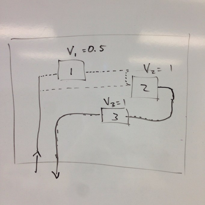
Forced Flow Law: Xi = Vi * X
Response Time Law: R = N/X – Z

Denning gives the example of a wine cellar to demonstrate the principle of Little’s law.  If a restaurant owner would like their wine to be aged R = 10 years, and they sell X = 7,300 bottles per year, the owner should build a wine seller with a Q = R * X = 73,000 bottle capacity.

Balance Equation

λ(n): Arrival rate when system is in state n.
μ(n): Completion rate when system is in state n.
p(n): Fraction of time system is in state n.

Balance Equation: For a system of states {0, 1, … n}, the balance equation is λ(n-1)p(n-1) = μ(n)p(n)

    ATM:

p(n) = p(n-1)λ/μ

Probability of dropping telephone calls:

λ: Arrival Rate
1/μ: Average Call Duration
nμ: Departure Rate

p(n) = p(n-1)λ/(nμ)

Probability of dropping a call is p(N+1) where N is the capacity.

Computing with Models (Multi-Server Models)

In 1973, Jeff Buzen discovered “Mean Value Analysis”, a way to calculate in O(#users * #servers) time the server response times, system response time, system throughput, and server queue lengths. The model is extended from the principles of the operation laws.