Introduction

————

Profiling repetitive behavior in programs has historically been difficult. “Active profiling” identifies program phases by controlling the input of the program, and monitoring the occurrences of basic blocks in execution.

There are two important definitions:

(1) Phase: “A unit of predictable behavior in that its instances, each of which is a continuous segment of program execution, are similar in some important respect.”

(2) Phase Marker: A basic block that, when executed, is always followed by an instance of the program phase it marks.

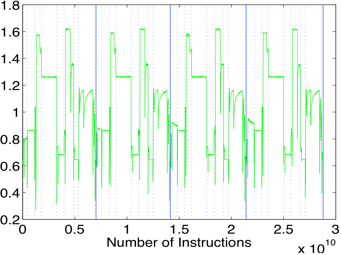
The above figure (Figure 2 in the paper) shows the IPC over logical time for GCC compiling a series of identical loops.

Selecting Phase Markers
———————–

The paper presents a 3-step method for identifying phase markers:

(1) The program is given a test input with f identical requests (e.g. in the figure compiling the same loop f times). Basic blocks which execute exactly f times are then selected as potential phase markers. Candidate phase markers whose inter-occurrence distances vary significantly are removed from consideration (because actual phase markers should occur at regular intervals).

(2) Analysis tests whether each remaining candidate occurs g times with other inputs that have g non-identical requests. If not, the candidate is removed from consideration.

(3) In step 3, inner-phases and their phase markers are identified.

Evaluation
———-

They test their system on 3 different programs with repetitive inputs, and show figures with phase markers for each:

(1) GCC: 4 identical functions.

(2) Compress: “A file that is 1% of the size of the reference input in the benchmark suite”. Compress has inherent repetition, because it compresses and decompresses the same input 25 times.

(3) L1: 6 Identical Expressions.

(4) Parser: 6 copies of a difficult-to-parse sentence.

(5) Vortex: A database and 3 iterations of lookups.

Uses of Behavior Phases
———————–

Garbage Collection: A behavior phase “often represents a memory usage cycle, in which temporary data are allocated in early parts of a phase and are dead by the end of the phase”. If garbage collection is run at the end of the phase, there is likely to be a higher fraction of garbage. Shen et al. implemented “preventive” garbage collection and applied it to the Lisp interpreter L1. (The standard “reactive” type of GC collects when the heap is full). Their testing results showed that preventive GC can result in faster execution times than reactive GC. However, in the test they showed, not using GC was faster than either of the GC options, so I’m not sure what to make of their result.

Memory Leak Detection: “If a site allocates only phase-local objects during profiling, and if not all its objects are freed at the end a phase, it is likely that the remaining objects are memory leaks.” This observation can be used to give programmers recourse to find memory leaks. Additionally, phase-local objects that are not freed by the end of the phase can be placed on the same virtual memory page. If not used, they will just go to disk, and not clog up memory.

Shuchang Zhou proposed a efficient algorithm to calculating the hit probability for cache with random replacement policy.

How much one cache can influence performance are often evaluated by running a cache simulator by collected traces. Different associativities, sizes and replacement policies will lead to different result. But for one special cache with random replacement policies, single round simulation can only gives one possible result of performance because of the randomness. So we have to run the simulation multiple times to get a average performance which is very inefficiency.

Based on this observation, they came up with a efficient way to calculate hit probability of each memory access by using expectation, which can be used to derive miss ratio.

Foundation:

      The trace of the accessed sequence (cache lines) is:

               a0, a1, a2, …, aN.

     The miss event of time i is Xi. if a miss event happens at i, then Xi = 1, else Xi = 0.

               X0, X1, X2, … XN.

      So the hit event will be 1-Xi at time i.

       Assume k is the time when the reuse window starts, the number of misses since k to time i will be Zi.

            If the reuse window exists,

                    Zi = sum(Xl), ( k+1<=l<= i-1 )

             Else,

                     Zi = infinite

      The expectation will be the following according to the linearity of expectation,

                     E(Zi) = sum( E(Xl) ) , ( k+1<=l<= i-1 ) or infinite

        With the definition number of misses Zi, E(Xi) can be defined as:

                       E(Xi) = 1 – E( (1-1/M)^Zi ), M is the cache size

         When M is very large,

                       E(Xi) ~ 1-(1-1/M)^E(Zi)

         Proof:

                        if Zi == infinite:

                                 1-(1-1/M)^E(Zi) = 1 – E( (1-1/M)^Zi ) = 0

                         Else:

      Then they proposed two algorithms to calculate E(Zi ) efficiently from E(Xi) and compared the results with average 5, 50, 500 round naive simulation which proves their method has less error.

Characterizing the memory performance of today’s diverse workloads is an important and challenging problem. Considering their bursty, irregular, and dynamic behavior along with limited available resource, achieving efficient and accurate characterization has been the focus of many research papers in the field.

Denning’s working set theory lead to the first abstraction for memory performance. Simply, extract the phases of a program and then compute the working set size of each program. With the development of caching memories, choosing the cache size became an important performance decision. This choice required a method that can approximate the program’s memory performance under different cache sizes; the miss ratio curve. However, at the time, the best practice for computing such a curve was Mattson’s original stack simulation algorithm, which required O(MN) time and O(M) space for a trace of N requests for M unique elements (a hash table is used for storing the last access times). An optimization using a balanced tree to maintain stack distances reduces the time complexity to O(N lg M), while it preserves the space cost.

It looks like efforts on further reducing the costs fail when we target the exact hit ratio curve. Zhong et al. [1] proposed computing the approximate stack distances. They design a new data structure, called a scale tree and use that to approximate the reuse distance of every request with relative precision. They reduce the time complexity to O(N lg lg M) while requiring the O(M) space as before.

It turns out the problem of estimating the stack distances is closely related to the distinct elements problem: How many distinct elements are in a stream? This well-studied problem is also known as cardinality estimation and zero frequency moment estimation (F0 estimation). Here is the approximation version of the problem.

Given δ>0 and ε>0, and a sequence of elements with M distinct elements (M is unknown), give C such that |M-C| < εM with probability at least 1-δ.

It is natural to ask the question of “how much space and time is necessary or sufficient for any algorithm with such guarantee.” It turns out that if δ=0 or ε=0 then the space cost is Ω(M). However, if none of these cases happen then the optimal space bound is Ө(lg M + ε^2) [3]. Here is a simpler algorithm that achieves a multiplicative guarantee. These algorithms are alternatively called probabilistic counters.

“Let d be the smallest integer so that 2^d > n, and consider the members of N as elements of the finite field F = GF(2^d), which are represented by binary vectors of length d. Let a and b be two random members of F , chosen uniformly and independently. When a member a_i of the sequence A appears, compute z_i = a · a_i + b , where the product and addition are computed in the field F . Thus z_i is represented by a binary vector of length d. For any binary vector z, let r(z) denote the largest r so that the r rightmost bits of z are all 0 and put r_i = r(z_i). Let R be the maximum value of r_i, where the maximum is taken over all elements a_i of the sequence A. The output of the algorithm is Y = 2^R. ” (adopted from [4])

This paper proposed a support for exploiting fine-grained data parallelism (SSE, AVX and GPU) for a set of applications which traverse multiple, irregular data structures (tree, NFA). There are two components in this support: 1. code generation: generating  code that exploits the platform’s support on fine-grained data parallelism in a portable manner. 2. locality optimization: optimize the memory layout to improve inter-thread and intra-thread locality.

The paper is well organized. It first introduced the class of applications (irregular applications with independent traversal) the proposed method targets and challenges in optimizing them (unbalanced workload, divergence, pointer-based traversal). It then specifies the platforms it targets on: x86 system with SSE instructions and NVIDIA GPUs. (SIMD platform). The introduction ends with a list of contributions.

First, code generation and execution. The author developed an immediate language to describe the traversal of the target applications. This immediate language is used to enable portability of the algorithm. A runtime scheduler is responsible to execute the bytecode and perform some necessary dynamic optimization. One specific optimization mentioned in the paper is stream compaction. Stream compaction basically compacts the valid output of a vectorized operation together by “bubbling” the invalid output. This technique, as claimed by the author, can be extended to the GPU platform, with modifications.

Second, optimized data layout. The data layout of irregular data structure is to linearize the data elements in memory. There are two goals here, as clearly specified by the author: 1. co-locating nodes (in the same cache line) that are likely to be accessed concurrently by different threads (inter-thread locality). 2. co-locating threads that are accessed in successive steps by the same thread (intra-thread locality).

Take the traversal of 4 trees as example. There are 5 primitive layouts proposed in the paper. DF and BF correspond to Depth-First and Breath-First, which layout one single tree’s nodes together in memory. LL means level-by-level. It layouts the nodes at the same level (across multiple trees) together in memory. It has better locality for vectorized operations than the first two strategies. SLL is Sorted level-by-level. The author observed that in some cases, during the left children are biased over the right children. Therefore it is beneficial to group the nodes which are left children of their parents together. CC is Cache-Concious. It has an idea that when a parent is traversed, its children may immediately be accessed. Therefore it is beneficial to group parent nodes with child nodes while still maintaining level-by-level layout. These five layouts can be combined to form a hybrid layout, which is, the top x levels use SLL while the rest levels use CC. The value of x is a user-defined parameter, called switching parameter.

The author then analytically described a formula to calculate x for LL-CC hybrid layout and SLL-CC hybrid layout. The model is to minimized cache misses and thus *execution time*. There are assumptions in this model. First, no temporal locality considered, which means one node is traversed exactly once. Second, a complete binary tree. Also, to test whether a certain bias on left/right child exists, sampling is used.

To shortly summarize their evaluation, they observed up to a 12X speedup on one SIMD architecture. They also get as much as 45% speedup over a suboptimal solution.

In his MS thesis published in Vancouver Canada four months earlier, Zachary Drudi reported the result of using the footprint technique developed by us to predict the hit ratio curve for a number of Microsoft traces, for cache sizes ranging from 0 to gigabytes (up to 1TB).  The footprint prediction is accurate in most cases.  Below is the plot copied from the thesis (page number 32, page 40), where avgfp is the footprint prediction, and mattson is the ground truth calculated from the reuse distance (LRU stack distance).

The author implemented our technique entirely on his own without consulting or informing any of us.

The thesis is titled A Streaming Algorithms Approach to Approximating Hit Rate Curves, available online from the University Of British Columbia.

(copyright Zachary Drudi, 2014)

In a series of papers in PPOPP 2008 (poster), PPOPP 2011, PACT 2011, and ASPLOS 2013, Rochester researchers have developed a set of techniques to measure the footprint and use it to predict other locality metrics including the miss/hit ratio curve and reuse distance, for exclusive and shared cache.  We have shown that the footprint techniques are efficient and largely accurate.  Mr. Drudi’s results provide an independent validation.

This is the first time we know that the technique is used in characterizing storage workloads.  The same implementation was used in their OSDI 2014 paper Characterizing storage workloads with counter stacks, J. Wires, S. Ingram, N. J. A. Harvey, A. Warfield, and Z. Drudi.

References:

[1] Yutao Zhong, Xipeng Shen, Chen Ding: Program locality analysis using reuse distance. ACM Trans. Program. Lang. Syst. 31(6) (2009)
[2] Jake Wires, Stephen Ingram, Zachary Drudi, Nicholas J. A. Harvey, Andrew Warfield: Characterizing Storage Workloads with Counter Stacks. OSDI 2014: 335-349
[3] Daniel M. Kane, Jelani Nelson, David P. Woodruff: An optimal algorithm for the distinct elements problem. PODS 2010: 41-52
[4] Noga Alon, Yossi Matias, Mario Szegedy: The Space Complexity of Approximating the Frequency Moments. J. Comput. Syst. Sci. 58(1): 137-147 (1999)
[Ren+:TACO14] A Portable Optimization Engine for Accelerating Irregular Data-Traversal Applications on SIMD Architectures