Assignment 6 (Dead Code Elimination)

This assignment is due Monday April 18th at 11:59pm.

For this assignment you are expected to identify and eliminate dead code. Dead code is any instruction that does not affect the output of the program (a function, in particular). For DCE (dead code elimination), you will need to use def-use chains to reason about instructions that do not affect the outputs. Remember that the output of a function is not limited to what it is returning.

IMPORTANT NOTE:

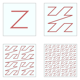
Those who implemented assignment 4 in LLVM, and have relied on the SSA property to find def-use chains with a linear scan of the LLVM-IR, are expected to implement a further requirement for this assignment, whether they are choosing URCC or LLVM for this assignment. That is Common Subexpression Elimination (CSE). An example of this optimization has been illustrated below.

CSE-example

Adopted from [1]

For CSE, you must first do the AVAIL analysis and then reason about expressions that are redundant.

Note 1: Since LLVM does not permit copy instructions, you may need to use the “ReplaceAllUsesWith” method to replace all uses of c with t. Also, since LLVM uses the SSA representation, you might need to insert new phi nodes.

Note 2: You do not need to implement partial redundancy elimination (PRE) for this assignment.

Testing

Your are expected to test your optimization pass by counting the number executed instructions. To do so, you are provided with a test script. Download this script into your URCC repository.

If you are using URCC for this assignment, you can easily run “./test.rb all” to run all the tests. You can also run an individual test by running “./test.rb #{program_name}”.

If you are using LLVM for this assignment, you will need to reimplement Test.test method in the script above by following the current implementation of that method. This is where you need to compile a program and apply your optimization, and instrumentation. You are allowed to use your peers’ test scripts.

The “./test.rb all” command will give you a “urcc_test_results.txt” file that includes the program outputs (along with your dynamic instruction count. Remember to print the instruction count as a single line “INST COUNT: x”, where x is the number of total executed instructions). Include this file in your report, along with your test script (if modified) and instructions on how to run the tests. Do not forget to give a thorough explanation about your implementation.

Note: URCC appears to be failing on generating a correct executable for two of the test cases: sort.c and tax.c. You can exclude these test cases by removing them from the test directory.

Assignment 5: Def-Use Chains

This assignment is due on Wednesday March 30th at 11:59pm.

In this assignment, you are expected to build the def-use chains for a program. You can either use your own CFG pass (if you are sure about its correctness), or adopt any correct CFG pass that is available to you.

Your output must have the following format. For every definition of a variable a, and for every use of a which is reachable from that definition (without any intervening def), you must output

[a, def, use],

where def and use are the program statements corresponding to the definition and use of a.

Run your analysis on the test cases provided in the URCC test directory and report the results. Explain your implementation and findings in a readme file. Archive everything and submit on blackboard.

Assignment 4: LVN in URCC/LLVM

For this assignment you are expected to implement the local value numbering optimization in URCC or LLVM. The requirements are the same as in assignment 1, except that the redundancy elimination part is now required. For this assignment, you don’t need to implement Stewart extension.

Test your optimization pass on URCC test cases. Report your implementation details and your findings in a readme file and submit on blackboard.

If you are working on LLVM, remember to turn off optimizations by using the “-O0” flag when emitting LLVM bitcode (The base project directory in /home/hoover/u1/cs255/cs255-llvm has been modified accordingly).

This assignment is due Sunday March 20th at 11:59pm.

Assignment 3 (CFG in URCC/LLVM)

In this assignment you will implement a pass to build a program’s CFG from its linear code. This assignment is due on Sunday March 6th at 11:59pm.

For this assignment, you can choose to use either the URCC compiler or LLVM.

Instructions for URCC

  1. Checkout and install the URCC compiler (follow the instructions in the README file). Make sure you are using a version of clang between 3.3 and 3.6 or URCC may fail. If you decide to use the CSUG machines, you can use clang 3.6 that is installed in /u/cs255/build-llvm-36/bin.
  2. Follow the algorithm in section 5.3.4 of the Cooper & Torczon book (page 241) to write a pass that builds the CFG of the program and visualizes it using graphViz (instructions on how to write a URCC pass are included in the README file).
  3. Test your compiler pass on test cases included in the test directory.
  4. Explain your implementation in a Readme file. Report all test case failures.
  5. Archive your code and the Readme file and submit on Blackboard.

Note: A CFG pass is already implemented in the URCC compiler. You shall not look at that implementation.

Instructions for LLVM

  1. Following the same instructions as in assignment 2, create an LLVM project in your CSUG account.
  2. Implement a pass that builds the CFG of the program and visualizes it using graphviz. If you need to iterate over instructions in a function, you must use the following code:
    #include "llvm/IR/InstIterator.h"
    
    // F is a pointer to a Function instance
    for (inst_iterator I = inst_begin(F), E = inst_end(F); I != E; ++I)
      errs() << *I << "\n";
  3. You can use BGL (Boost Graph Library), which is already installed on CSUG filesystem. Graphviz is included in this library.
  4. Test your compiler pass on test cases included in URCC’s repository (https://github.com/dcompiler/urcc/tree/master/tests).
  5. Explain your implementation in a Readme file. Report all test case failures.
  6. Archive your code and the Readme file and submit on Blackboard.

Note: A CFG pass is already implemented in LLVM. You shall not look at that implementation.


Assignment 2 (GCC/LLVM)

In this assignment, you will implement and test a compiler pass that instruments a program to report the number of intermediate-level executed instructions. You can choose to implement this pass either in gcc or llvm. For your convenience, these two compilers are already installed on the csug network.

The idea is to insert appropriate calls in the program (instrumentation).

*********************************Instructions on GCC****************************************
——————————————————————————————–
Log in to your csug account.
$ cp -r /u/cs255/cs255-gcc YOURUSERNAME-cs255-gcc
$ cd YOURUSERNAME-cs255-gcc

Included files:
———————–
* inst-cnt-plugin.cc
You must implement your compiler pass here.
This file already provides the skeleton and a related example.

* inst-cnt-rt.c
This file implements the runtime functions that you need for the instrumentation.

* test.c
This is a simple program to test your pass.

After implementing the pass, compile it by running “make” and test it using “make check”. This gives you the instrumented program “test”. Run it on the string “cs255” and report your output. Make sure to explain your implementation and findings in a readme file.

Submission guideline:
Archive your working directory using the following command line, and submit on Blackboard.
tar -czvf YOURUSERNAME-cs255-gcc.tar.gz YOURUSERNAME-cs255-gcc/

Note: you can use the gcc option -fdump-tree-all to inspect your instrumentation at the GIMPLE level. After running “make check” with this option, look for the file which has your pass name as a suffix in its filename.

*********************************Instructions on LLVM**************************************
——————————————————————————————–
Log in to your csug account.
$ cp -r /u/cs255/cs255-llvm YOURUSERNAME-cs255-llvm
$ cd YOURUSERNAME-cs255-llvm

Included files:
———————–
* lib/InstCounter.cpp
You must implement your compiler pass here.
This file already provides the skeleton and a related example.

* runtime/InstCounting.c
This file implements the runtime functions that you need for the instrumentation.

* test/test.c
This is a simple program to test your pass.

After implementing your pass, compile it by running “make” in your top-level directory. Then cd into the “test” directory and run “make check” to test your pass. This gives you the instrumented program “test”. Run it on the string “cs255” and report your output. Make sure to explain your implementation and findings in a readme file.

Submission guideline:
Archive your working directory using the following command line, and submit on Blackboard.
tar –exclude=’.svn’ –exclude=’autoconf’ -czvf YOURUSERNAME-cs255-llvm.tar.gz YOURUSERNAME-cs255-llvm/

Note: you can use the llvm-dis tool (/u/cs255/build-llvm-38/bin/llvm-dis) to check your instrumentation at IR level. Run this tool on the llvm bitcode file that is generated by your pass:
/u/cs255/build-llvm-38/bin/llvm-dis <test.bc.opt> test.bc.opt.ll
———————————————————————————————

CS255 Assignment #1 (LVN)

In this assignment, you are asked to implement local value numbering (LVN) and check for redundant expressions.

You are expected to handle commutativity for commutative operations. Recall that an operation is commutative if you can change the order of operands without changing the result. For example (+) is commutative but (-) is not. Your implementation must be able to assign the same value number to a+b and b+a.

As the final requirement, improve LVN by adding the Stewart extension. The Stewart extension improves LVN by identifying additional redundancy in the following example form.

a = b + c

d = a – b

Specifically, it guides LVN to assign the same value number to both (c) and (d). The idea of the solution was first raised by Chris Stewart when he was taking the class around 2004.  His idea was to insert additional value relations into the value number table. You should first work out this idea and make it concrete as an extension to the basic value numbering algorithm.

Note 1: You are expected to apply the Stewart extension on four operations: ‘+’, ‘-‘, ‘*’, and ‘/’.

Note 2: You should make sure that the Stewart extension can be applied on the following code as well.

a = b + c

e = a

d = e – b


To complete this assignment, take the following steps:

1. From Blackboard, download block.rb and vn_tests.rb to your project directory.

2. Implement the LVN class in the new file vn.rb.

4. Make sure all the tests in vn_tests.rb pass.

5. Document any test failures, if there is any, and explain why, in README.txt in plain text.

6. Extra credit.  In addition to finding the statements with a redundant expression, generate optimized code where all redundant expressions are removed.  Demonstrate the optimizer with a set of tests and put them in opt_tests.rb.  The tests should include all three tests in vn_tests.rb.

7. Submit your assignment on Blackboard. Make sure to include all the ruby files in your submission.

Due time: Friday Jan 29th at 23:59:59 EST.

Late submission policy: Each student can have a total of two days used for late submissions over all assignments . This means that if you submit the LVN assignment on Sunday, you will not be able to do any other late submission. But if you submit on Saturday, you still have one more day to use for one other assignment.

Policy on academic honesty :  Every line of code of the LVN analyzer and optimizer must be written by the student.  Do not copy code.  Do not show your LVN code to others until 2 days (48 hours) past the assignment due time.  The teaching staff is required to report every violation of the policy or suspicion of violation to the university’s Academic Honesty Board.  Contact the teaching staff if you have questions on the policy.


Efficient Computation of Reuse Distance

Characterizing the memory performance of today’s diverse workloads is an important and challenging problem. Considering their bursty, irregular, and dynamic behavior along with limited available resource, achieving efficient and accurate characterization has been the focus of many research papers in the field.

Denning’s working set theory lead to the first abstraction for memory performance. Simply, extract the phases of a program and then compute the working set size of each program. With the development of caching memories, choosing the cache size became an important performance decision. This choice required a method that can approximate the program’s memory performance under different cache sizes; the miss ratio curve. However, at the time, the best practice for computing such a curve was Mattson’s original stack simulation algorithm, which required O(MN) time and O(M) space for a trace of N requests for M unique elements (a hash table is used for storing the last access times). An optimization using a balanced tree to maintain stack distances reduces the time complexity to O(N lg M), while it preserves the space cost.

olkenIt looks like efforts on further reducing the costs fail when we target the exact hit ratio curve. Zhong et al. [1] proposed computing the approximate stack distances. They design a new data structure, called a scale tree and use that to approximate the reuse distance of every request with relative precision. They reduce the time complexity to O(N lg lg M) while requiring the O(M) space as before.

scale

It turns out the problem of estimating the stack distances is closely related to the distinct elements problem: How many distinct elements are in a stream? This well-studied problem is also known as cardinality estimation and zero frequency moment estimation (F0 estimation). Here is the approximation version of the problem.

Given δ>0 and ε>0, and a sequence of elements with M distinct elements (M is unknown), give C such that |M-C| < εM with probability at least 1-δ.

It is natural to ask the question of “how much space and time is necessary or sufficient for any algorithm with such guarantee.” It turns out that if δ=0 or ε=0 then the space cost is Ω(M). However, if none of these cases happen then the optimal space bound is Ө(lg M + ε^2) [3]. Here is a simpler algorithm that achieves a multiplicative guarantee. These algorithms are alternatively called probabilistic counters.

“Let d be the smallest integer so that 2^d > n, and consider the members of N as elements of the finite field F = GF(2^d), which are represented by binary vectors of length d. Let a and b be two random members of F , chosen uniformly and independently. When a member a_i of the sequence A appears, compute z_i = a · a_i + b , where the product and addition are computed in the field F . Thus z_i is represented by a binary vector of length d. For any binary vector z, let r(z) denote the largest r so that the r rightmost bits of z are all 0 and put r_i = r(z_i). Let R be the maximum value of r_i, where the maximum is taken over all elements a_i of the sequence A. The output of the algorithm is Y = 2^R. ” (adopted from [4])

Recently, Wires et al. [2] have used these probabilistic counters to approximate the hit ratio curve and achieved sublinear space.

References:

[1] Yutao Zhong, Xipeng Shen, Chen Ding: Program locality analysis using reuse distance. ACM Trans. Program. Lang. Syst. 31(6) (2009)

[2] Jake Wires, Stephen Ingram, Zachary Drudi, Nicholas J. A. Harvey, Andrew Warfield: Characterizing Storage Workloads with Counter Stacks. OSDI 2014: 335-349

[3] Daniel M. Kane, Jelani Nelson, David P. Woodruff: An optimal algorithm for the distinct elements problem. PODS 2010: 41-52

[4] Noga Alon, Yossi Matias, Mario Szegedy: The Space Complexity of Approximating the Frequency Moments. J. Comput. Syst. Sci. 58(1): 137-147 (1999)

Improving Locality via Space Filling Curves (Chatterjee+: ICS99, Jin-Mellor:TMS05, Frens-Wise:PPOPP03)

“In 1877 Cantor demonstrated that there is a bijective function between any two smooth manifolds independent of their dimension. This in particular showed that such functions between the unit interval and the unit d-cube for d >1 exist. In 1879 Netto proved that if the dimensions of the manifolds are different such a function is necessarily discontinuous. The question whether a surjective, continuous map from the unit interval to the unit square exists remained open. In 1890 Peano answered this question positively by presenting such a map, now known as Peano (space-filling) curve.”

Peano Curve (from Wikimedia)

Early after, in 1891, Hilbert discovered a simpler variant of the Peano Curve, now known as Hilbert Curve.

Several Iterations of Hilbert Curve

Several Iterations of Hilbert Curve

Both Peano and Hilbert curves require rotations. Here’s the Morton (Z-order) curve which doesn’t.

Morton (Z-order) Curve

Morton (Z-order) Curve

Space filling curves have the following properties which make them appealing for locality improvement.

  1. Space-filling: They are continuous functions whose range comes arbitrary close to a given point in the n-dimensional space. Thus they preserve locality at any granularity, regardless of the dimensionality.
  2. Dimensionality: They exist for all dimensions greater than one.
  3. Self-similar: They can and are usually defined as non-terminating recurrences.

However, when space-filling curves are used to improve data layout, traversal or indexing of the curve must be efficient. Programming languages often lack support for any indexing other than the canonical one, since they are not as simple to implement. Under the canonical indexing, the relative address of the array element A[i, j] is simply equal to i × n + j, where n is the length of the first dimension of the array. This is efficient to implement in hardware. Furthermore, because this formula is linear, it is easy to compute the address of an element relative to another element in the same row or column. Therefore, in linear traversals of the array, we can avoid the cost of multiplication in the above formula.

Jin and Mellor-Crummey (TMS05) developed a universal turtle algorithm to traverse various space-filling curves using each curve’s movement specification table. They used the same approach to transform the coordinates of a point into its position along the curve (indexing).  Interestingly, it turns out that in a Morton curve, the conversion from the canonical index to the Morton index can be carried out in a much more efficient way, by interleaving the bits of the indices.

Research shows that the choice of layout is critical for performance. Frens and Wise designed a QR factorization algorithm specialized for Quadtree layout (a layout very similar to Z-order curve) and showed that not only does it improve reuse but it also improves parallelism due to the reduction in false sharing. Here is a graph illustrating their speedup on a uniprocessor system.

Frens-Wise: PPOPP03

Frens-Wise: PPOPP03

2015/03/img_7768.jpg

3D view from vismath.eu

hilbert-kurve-3d-modell-raum

Algorithms For Memory Hierarchies (Meyer+): the external memory model and the cache oblivious model

The increasing gap between memory latency and processing power requires a model under which we can decompose
these two. This book discusses models of memory hierarchy that suit this purpose.

The simplistic “external memory model” models the memory hierarchy as an internal fast memory and an external memory. The CPU operates on the internal memory. The external memory can only be accessed using I/Os that move B contiguous words between internal and external memory. The number of these I/O transfers defines the performance of an algorithm under this model, while the CPU performance is defined by the processing work on the internal memory.

emm

The external memory model

In a real memory hierarchy, a hardware cache uses a fixed strategy to decide which blocks are kept in the internal memory, whereas the external memory model gives the programmer full control over the content of the internal memory. This difference will probably not have devastating consequences as prior work has shown that in practice we can even circumvent hardware replacement schemes.

It is important to design algorithms that perform efficiently under this model. A relatively simple example illustrated in the book is implementing a stack. A naive implementation of the stack leads to O(N) transfers between internal and external memory in the worst case, where N is the number of stack operations (push and pop). However, using a buffer of size 2B (B being the block size), we can achieve amortized performance of O(N/B).

The book designs and analyzes efficient algorithms for several other fundamental problems such as sorting, permuting, and matrix multiplication.

The second model is the “cache oblivious model.” Algorithms designed for the external memory model need to know parameters of the memory hierarchy in order to tune performance for specific memories. Cache oblivious algorithms, on the other hand, don’t have any knowledge of the parameters M (cache size) and B (block size). Further, it assumes that the internal memory is ideal (a fully-associative cache with optimal replacement policy).

An example illustrated in the book is the “Van Emde Boas Layout” for binary search on balanced trees.

“Given a complete binary tree, we describe a mapping from the nodes of the tree to positions of an array in memory. Suppose the tree has N items and has height h = log N + 1. Split the tree in the middle, at height h/2. This breaks the tree into a top recursive subtree of height ⌊h/2⌋ and √N several bottom subtrees B_1 , B_2 , …, B_k of height ⌈h/2⌉. There are √N bottom recursive subtrees, each of size √N. The top subtree occupies the top part in the array of allocated nodes, and then the B_i’s are laid out. Every subtree is recursively laid out.”

A view of the recursive layout

A view of the recursive layout

We now can analyze the number of cache misses for a binary search operation on a tree with a Van Emde Boas layout. If we denote by c(h) the number of cache misses on a tree of height h, we have:

c(h) = 2c(h/2) if h> lg(B)
c(h) <= 2 if h<= lg(B)

Therefore, we have c(h) = h – lg(B), which is lg N – lg B where N is the total number of nodes in the tree.

[Petrank and Rawitz: POPL02] The Hardness of Cache Conscious Data Placement

Data layout is critical for cache performance. An example of a poor data layout is one that maps frequently accessed data to the same set, which leads to an increase in conflict misses.

This famous piece of work by Petrank and Rawitz formally defines the problem and shows that computing the optimal data layout is extremely difficult, even if the full memory access sequence is known upfront. They study the problem in a cache conscious setting (all the cache parameters are known). The optimal data layout is a one-to-one mapping from data objects to the memory that gives the smallest number of cache misses.

For a t-way set associate cache of size k (a general specification of the cache), the paper calls the problem “minimum t-way k-cache misses.”

The paper proves that for any polynomial data layout algorithm there are sequences onwhich the algorithm performs extremely poorly. Specifically, it shows that for any e>0 there exists a “villain” sequence for which the data layout provided by the algorithm leads to more misses than a factor of N^(1-e) of the optimal (N is the length of the sequence).

The authors provide a reduction from the NP-hard “graph k-colorability” problem which is defined as follows.

Given a graph G, and k, is G k-colorable? i.e., does there exist a vertex coloring that leaves no monochromatic edges in the graph (edges that have both their endpoints colored the same are called monochromatic edges)?

Here is a sketch of the proof for a direct-mapped cache of size k.

For every instance of the graph k-coloring problem, we construct an instance of the minimum k-cache miss problem. For every vertex in the graph, we associate one memory object. For every edge we construct a memory access subsequence. Finally, we concatenate the subsequences to construct to full sequence. The key idea is to ensure that mapping the memory objects corresponding to the endpoints of an edge to the same location in the cache would incur a number of conflict misses that is polynomially related to the number of edges in the graph. This would guarantee that there is a huge gap between a data layout which corresponds to a valid k-coloring of the graph and one that is not. Therefore, if we are able to efficiently give a data layout that is within a decent bound of the optimal, we would be able to solve the k-coloring problem as well.

Following the same idea, the case can be proved for the general t-way set associative cache. The only difference is that in order to ensure the gap, we need to introduce more objects in the subsequences associated with the edges.

In the light of the negative result, a question is “how close we can get to the optimal layout?”. The authors present an algorithm that guarantees a data placement that always leads to a number of misses within a factor of (n/log n) of the optimal.