[Denning+:Acta_Informatica76] Optimal Multiprogramming

Optimal Multiprogramming
Denning, Kahn, Leroudier, Potier, Suri

In this paper, the authors give three memory-based techniques for maximizing throughput in a multiprogrammed system. “n” is the number of processes sharing processor time, or the “load”, and T(n) is the throughput.

First they develop a model for their system.

Model

a_i is the request rate for station i, and b_i is the service completion rate for station i. q_i is the fraction of departures from the processor that go to station i (q_0 is a departure). Station 1 is the paging device, so the page swap time is 1/b_1.

A couple of relationships:

b_0 = a_0 + … + a_m (there are m stations)

L(n) = 1/a_1 (system lifetime is average time between page faults)

q_i = a_i/b_0 (by definition, access rate at i / completion rate of processor)

T_i(n) is the throughput at station i. T(n) = T_0*q_0 (output rate of processor * fraction of that that leaves system).

“Three Load Control Rules”
————————–
(1) The Knee Criterion
– Throughput is maximized when memory space-time per job is minimized. In a lifetime curve, the knee is the point that minimizes the memory space-time due to paging. This can be done by managing the memory so that the sum of working set sizes is near the knee.

Screen Shot 2015-04-30 at 9.55.30 AM

(2) L = S Criterion
– L is system lifetime, and S is swap time. When the lifetime (time between page faults) is greater than the swap time (time to satisfy a page fault), this prevents queueing at the paging device, which would make it a bottleneck. This rule can be enforced by management of the memory, or by management of the load.

(3) 50% Criterion
– The idea here is to keep the paging device busy between 50% and 60% of the time. This can be enforced by managing the load.

Hao Luo 6 Month Review

Background. Multicore applications share cache. Composable analysis is needed to see how programs interact with dynamic, usage based cache management. Miss ratio/rate doesn’t compose.

Xiaoya’s work. Footprint composes but assumes uniform interleaving.

Jake et al. Common logical time in CCGrid 2015 handles non-equal length component traces, eg. one thread accesses memory 100 times more frequent than another thread. But we still assume uniform interleaving.

Hao repots several advances.

Time-preserving decomposition

Now we can compose threads that have any type of interleaving.

Cache associativity modeling

The Smith method is the dominant solution for nearly 40 years but assumes equal probability of access in all cache sets. Hao’s new solution removes this assumption and uses time-preserving decomposition to also allow non uniform interleaving.

GPU texture cache

Modeled as a sector cache to give composable performance for all cache sizes and associativity as for normal cache.

New studies

Space efficient algorithms for shared footprint analysis.

Possibly memcached or io traces.

Static locality analysis.

Locality aware scheduling

2015/04/img_8535.jpg

3 Techniques of Tree Sampling

At the 2015 University Day organized in the Systems workshop organized by Wang Chen at IBM Toronto, José Nelson Amaral of University Alberta gave a talk explaining the following studies.  The problem is estimating the size of a tree by traversing some but not all nodes.

“Mathematics of computation” by Donald Knuth in American Mathematical Society 1975 gave a sampling solution: Go down random tree paths to the leaves, and take the average of the sampled sub-tree size as the actual average sub-tree size.

Heuristic sampling by Peng Chen in 1992 takes samples but reuses the past results.  It uses the term Stratification but the technique sounds like memoization.  An example is the Fibonacci series.

The Alberta work is to estimate the number of leaf tasks in a recursive fork-join (Cilk) program.  The solution is a complete exploration of the top of the tree until it has the nodes 10 times the number of processors.  Then it uses the Knuth method to estimate the size of a sub-tree.

Another example is 3×3 puzzle, 181,440 states and 4×4, more than 10^13 states.

[Xipeng’s group ICS 2015] SM-centric GPU Scheduling and Locality-based Task Grouping

Currently GPU has a thread-centric model, where a task is the work specified by kernel(thread block ID).  There two important questions: When to schedule, which software can control through persistent threads, and where to schedule, which is the problem studied in this paper.  It groups tasks that share data.

Task co-location is important for locality and for resource utilization.  Improper concurrent execution of kernels leads to resource conflicts, e.g. too much shared memory/register demand so another kernel cannot be run.

The solution is SM centric.  A worker is started by hardware to run tasks from a queue, controlled by software.  The paper has a scheme to start the same number of workers on each SM.  In comparison, the past work on persistent threads can only run one worker per SM.

For irregular application, the paper uses GPU to parallel partition the data/tasks into locality groups.

Measured the effect in Co-run ANTT speedup = mean( default Ti / opt Ti), (average normalized turnaround time) and Co-run throughput.

Adriaens+:HPCA12’s study of co-run kernels.

[Crummey+:ICS99]Improving memory hierarchy performance for irregular applications

John Mellor-Crummey from Rice University investigated data and computation reordering to improve memory performance for applications with irregular memory accesses.

For regular memory accesses, the gap between CPU and memory can be well bridged by loop blocking and prefetching. but for irregular memory accesses, the accesses can only be known during the run time. One approach to improve memory performance is to dynamically reorder data before time consuming computations. And also, computation reordering along with data reordering will be much more effective. The reason why the data and computation reordering can be effective is that they increase the probability that data in the same block will be access closely in time and the probability that data will be reused before the block is elected.

For example, N-body is a classical irregular application which is used to calculate the interaction between particles. It contains two list, one stores the information of each particles and the other stores the paired indices of particles which will interact with each other.

f1.001

Data reordering can increase spacial locality by placing the data near one another by the accessed order. Two data reordering approaches are proposed:

First Touch Data Reordering(FTDR): before computation, a linear scan will be performed on the interaction list to get the new order for particle list.

f2.001

Space Filling Curve Data Reordering(SFCDR):  before computation, reordering the particle list by space filling curve which make the particles with shorter distance in space close with each other. And one advantage compared with FTDR, the space filling cure reordering can be performed without knowing the order of the computation.

f3.001

Computational reordering can improve spacial locality as data reordering and also improve temporal locality. Two computational reordering are proposed:

Space Filling Curve Computation Reordering(SFCCR):  reorder the computations according to space filling curve, and the particle list maintains the same.

f4.001

Computational Reordering by Blocking(CRB): Before reordering the computations, data should be given a block index (the index can be more than one dimension), then reorder the computations according to the block number which the particles belongs to the same block will be processed together.

f5.001

[Waldspurger+:FAST15]Efficient MRC Construction with SHARDS

[FAST15]Carl A. Waldspurger, Nohhyun Park, Alexander Garthwaite, and Irfan Ahmad, CloudPhysics, Inc.

This paper proposed a sampling based miss ratio curve construction approach. It focus on reducing memory complexity of other algorithms from linear to constant.
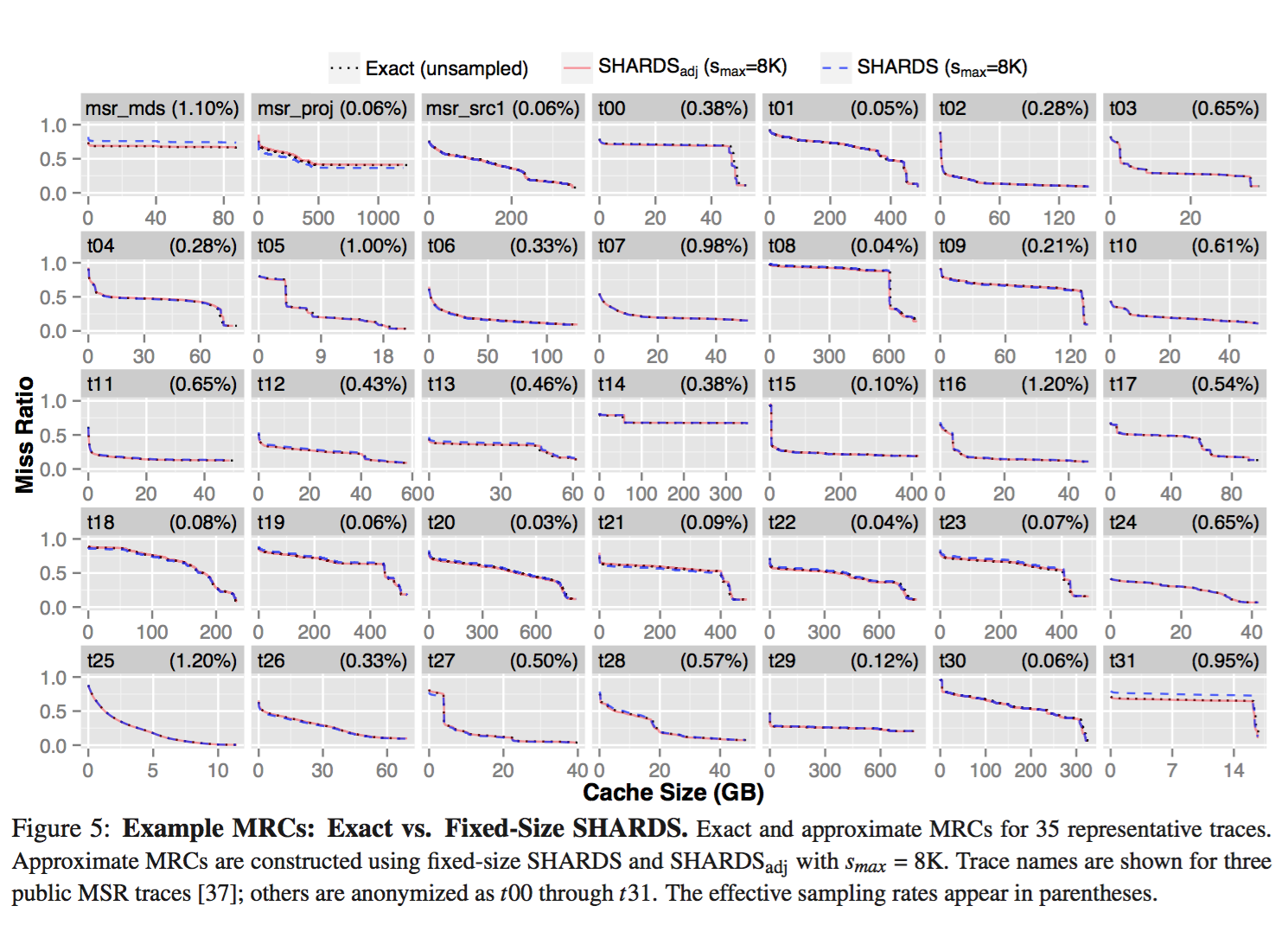
Evaluation on commercial disk IO traces show it has a high accuracy with a low overhead.

Motivation

Algorithms for exact miss ratio curve usually consume a huge amount of memory, which is linear to unique reference(counted as M). Thus when M becomes dramatically huge, the memory overhead becomes a big problem. In this paper, authors analyzed VMware virtual disk IO data which is collected from commercial cloud, the size of disks are from 8GB to 34TB, with a median of 90GB. This size reflects range of M.

Thus authors propose a two phases spatial sampling algorithm to reduce space complexity, including sampling on address and an algorithm to restrict size of sampling.

Algorithm and Implementation

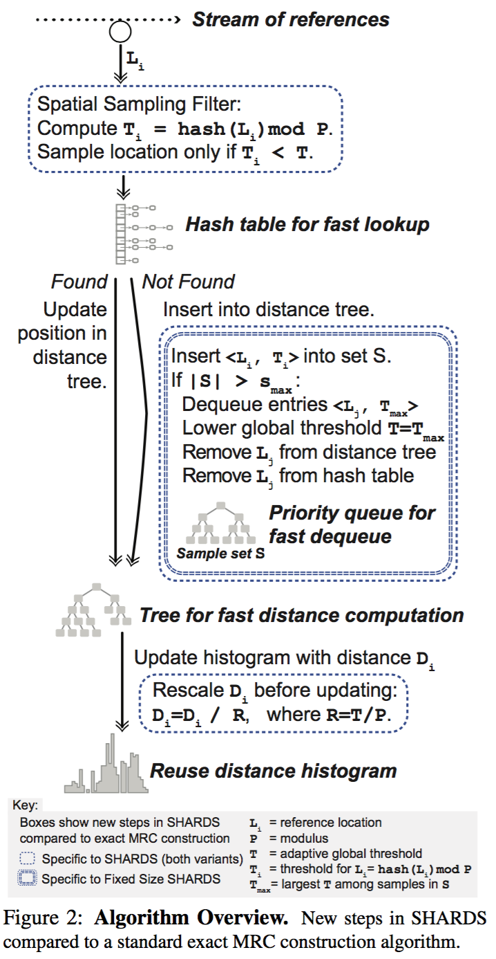
The algorithm contains 3 steps:

  1. sampling on addresses
  2. maintain fixed number of sampled addresses
  3. figure out reuse distance histogram while sampling

Algorithm of SHARDs

Sampling on address

For each address L, if hash(L) mod P < T, then this address is sampled. Thus sampling rate R = T/P.

Fixed number of address

Space complexity becomes M*R, and the objective is maximize R while M*R is less than specific boundary. But it is difficult to predicate M at runtime, thus it might not be a good decision to fix R at beginning of execution. Which means, it is necessary to adjust R at runtime, aka, decreasing R.

The approach is keeping a set S, which keeps all sampled values and their hash values, say for each address L[i], remember (L[i],T[i]). If |S| > S_max, then keep removing the one whom has maximal T[i] until |S| equal to S_max, and always let sampling boundary T = max(T[i]), where L[i] belong to S.

Reuse distance histogram

Reuse distance is computed with traditional approach, such as splay tree.

Since addresses space is sampled with rate R, thus the reuse distance is also scaled by R. For example, if distance d is gained through sampling, then before accumulating the histogram, d should be scaled to d/R.

Furthermore, since T will be adjusted according to previous section, and R = T/P, which means R will be adjusted at runtime, thus each time R is changed, the histogram should be rescaling again. In detail, all distance of the histogram should be multiplied by R_new/R_old.

Evaluation

Data is collected by SaaS caching analytics service which “is designed to collect block I/O traces for VMware virtual disks in customer data centers running the VMware ESXi hypervisor”. “A user-mode application, deployed on each ESXi host, coordinates with the standard VMware vscsiStats utility [1] to collect complete block I/O traces for VM virtual disks.” In addition, the data is composed of 16KB sized block, and cached with LRU algorithm.

Experiments results from paper

Appendix

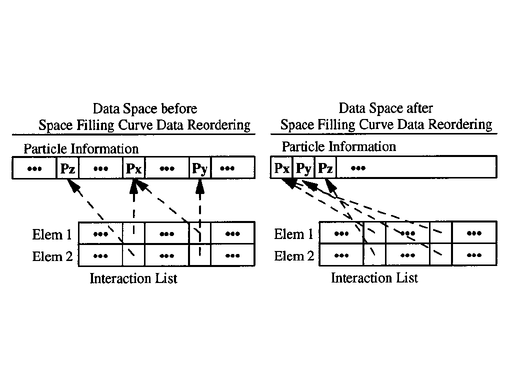
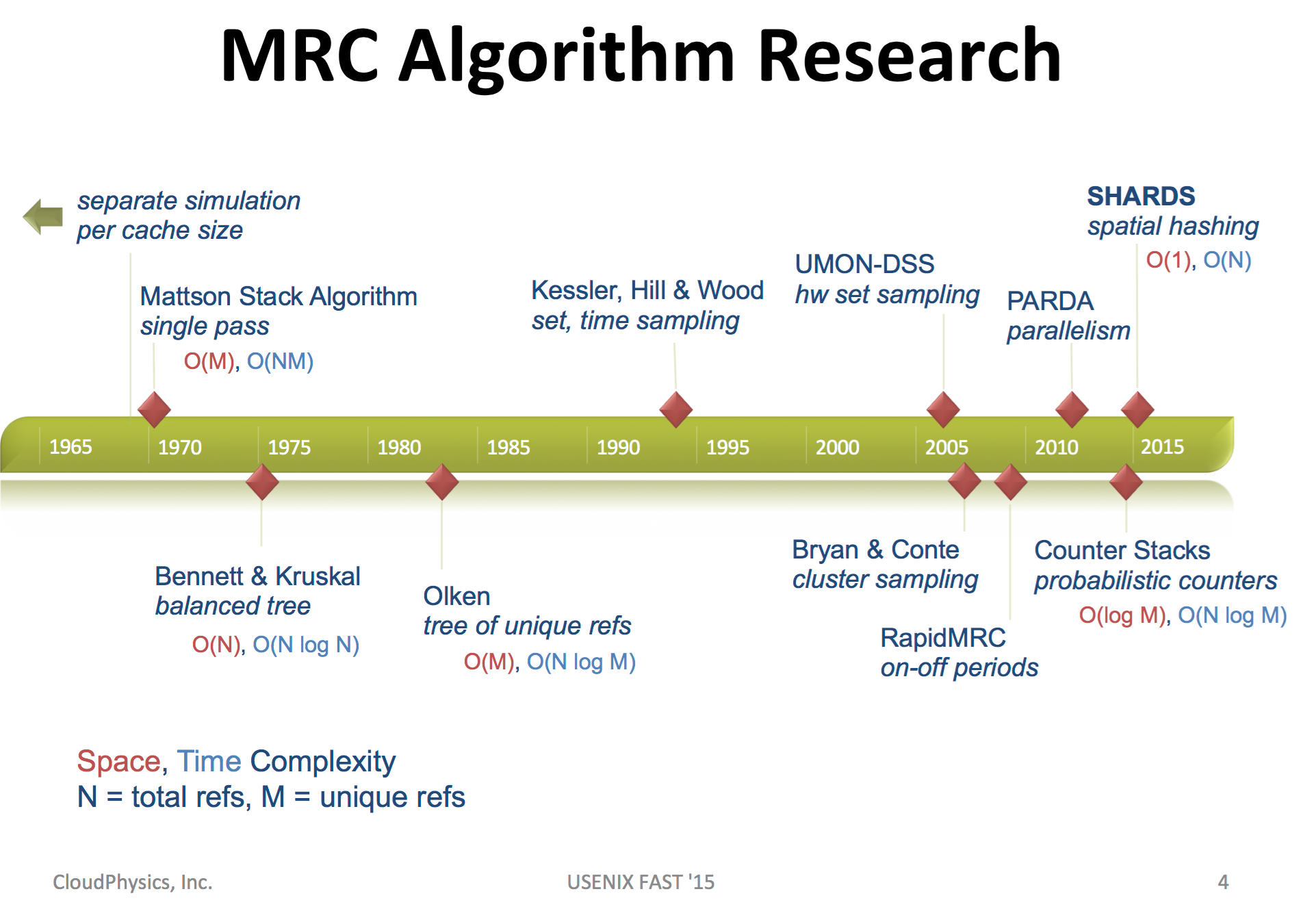
A great timeline comes from slides

Comes from Waldspurger etc. 's slides

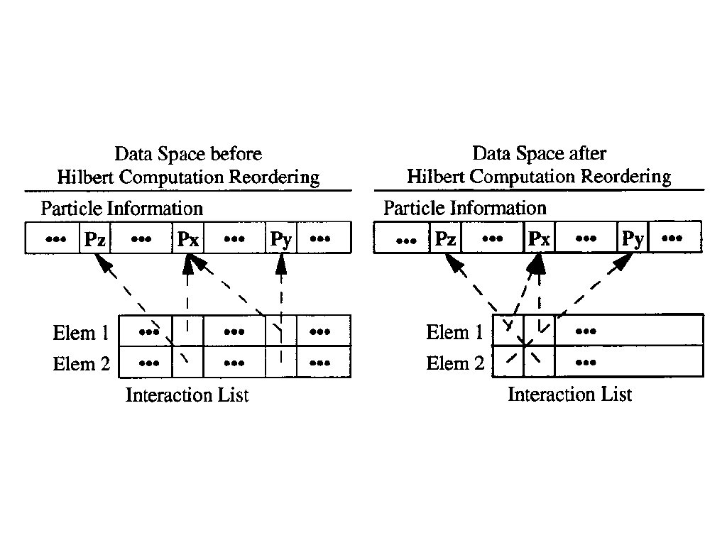
Comes from Waldspurger etc. ‘s slides

How about temporal sampling

“Use of sampling periods allows for accurate measure- ments of reuse distances within a sample period. How- ever, Zhong and Chang [71] and Schuff et al. [45, 44] ob- serve that naively sampling every Nth reference as Berg et al. do or using simple sampling phases causes a bias against the tracking of longer reuse distances. Both ef- forts address this bias by sampling references during a sampling period and then following their next accesses across subsequent sampling and non-sampling phases.”


[RutarH13] Software techniques for negating skid and approximating cache miss measurements

Modern hardware counters are used to find program instructions that cause most cache misses for example, and the way is to measure how many times a counter overflow happens on a particular instruction. However, when an overflow happens as an interrupt, the exact instruction causing the interrupt may be incorrect, a problem that Intel calls a “skid”.

The solution is to consider surrounding instructions as the set of probabilities. Then the overlap of these probabilities will show the most likely instruction.

The problem and solution are hardware dependent.

[Callahan+:JPDC88,DingK:IPDPS00] Program/machine Balance

To model performance, it is necessary to quantify the tradeoff between computation and communication, in particular, between the processing throughput and the data transfer bandwidth. The classic model is the notion called balance by Callahan, Cocke and Kennedy [JPDC 1988]. A balance is the ratio between the peak computing throughput and the peak data transfer bandwidth. It is known in the multicore era as the roofline model [Williams et al. CACM09] and has been known since earlier times as byte per flop.

If a machine is not balanced because the memory is not fast enough, a processor can achieve at most a fraction of its peak performance.

Both a program and a machine have balance. Program balance is the amount of the memory transfer, including both reads (misses) and writes (writebacks) that the program needs for each computation operation; machine balance is the amount of memory transfer that the machine provides for each machine operation at the peak throughput. Specifically, for a scientific program, the program balance is the average number of bytes that must be transferred per floating-point operation (flop) in the program; the machine balance is the number of bytes the machine can transfer per flop in its peak flop rate.

On machines with multiple levels of intermediate memory, the balance includes the data transfer between all adjacent levels [Ding and Kennedy, IPDPS00].

The paper tests the performance of two simple loops on SGI Origin2000 and HP/Convex Exemplar.  The first loop takes twice as long because it writes the array to memory and consequently consumes twice as much memory bandwidth.


double precision A[2000000]

for i=1 to N
A[i] = A[i]+0.4

end for

for i=1 to N
sum = sum+A[i]
end for

The paper shows the balance on an SGI Origin2000 machine. For example, convolution requires transferring 6.4 bytes between the level-one cache (L1) and registers, 5.1 bytes between L1 and the level-two cache (L2), and 5.2 bytes between L2 and memory. For each flop at its peak performance, the machine can transfer 4 bytes between registers and cache, 4 bytes between L1 and L2, but merely 0.8 bytes between cache and memory. The greatest bottleneck is the memory bandwidth, the ratio 0.8/5.2 = 0.15 means that the CPU utilization is at most 15%.  Note that prefetching cannot alleviate the bandwidth problem because it does not reduce the aggregate volume of data transfer from memory. In fact, it often aggravates the bandwidth problem by generating unnecessary prefetches.

Our earlier work has studied loop fusion and array regrouping [Ding and Kennedy, JPDC 2004] and run-time computation reordering and consecutive packing (data reordering) [Ding and Kennedy, PLDI 1999] to reduce the total bandwidth requirement of a program.  There are excellent follow up studies, which would be good to review later.