Existing Policies

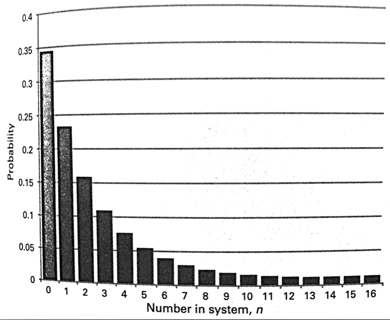
In their 1976 paper “VMIN — An Optimal Variable-Space Page Replacement Algorithm”, Prieve and Fabry outline a policy to minimize the fault rate of a program at any given amount of average memory usage (averaged over memory accesses, not real time).  VMIN defines the cost of running a program as C = nFR + nMU, where n is the number of memory accesses, F is the page fault rate (faults per access), R is the cost per fault, M is the average number of pages in memory at a memory access, and U is the cost of keeping a page in memory for the time between two memory accesses. VMIN minimizes the total cost of running the program by minimizing the contribution of each item: Between accesses to the same page, t memory accesses apart, VMIN keeps the page in memory if the cost to do so (Ut) is less than the cost of missing that page on the second access (R).  In other words, at each time, the cache contains every previously used item whose next use is less than τ = R accesses in the future. Since there is only one memory access per time step, it follows U that the number of items in cache will never exceed τ. Since this policy minimizes C, it holds that for whatever value of M results, F is minimized. M can be tuned by changing the value of τ.

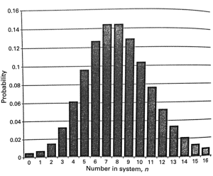
Denning’s working set policy (WS) is similar.  The working set W (t, τ ), at memory access t, is the set of pages touched in the last τ memory accesses. At each access, the cache contains every item whose last use is less than τ accesses in the past. As in the VMIN policy, the cache size can never exceed τ.  WS uses past information in the same way that VMIN uses future information. As with VMIN, the average memory usage varies when τ does.

Adaptations to Heterogeneous Memory Architectures

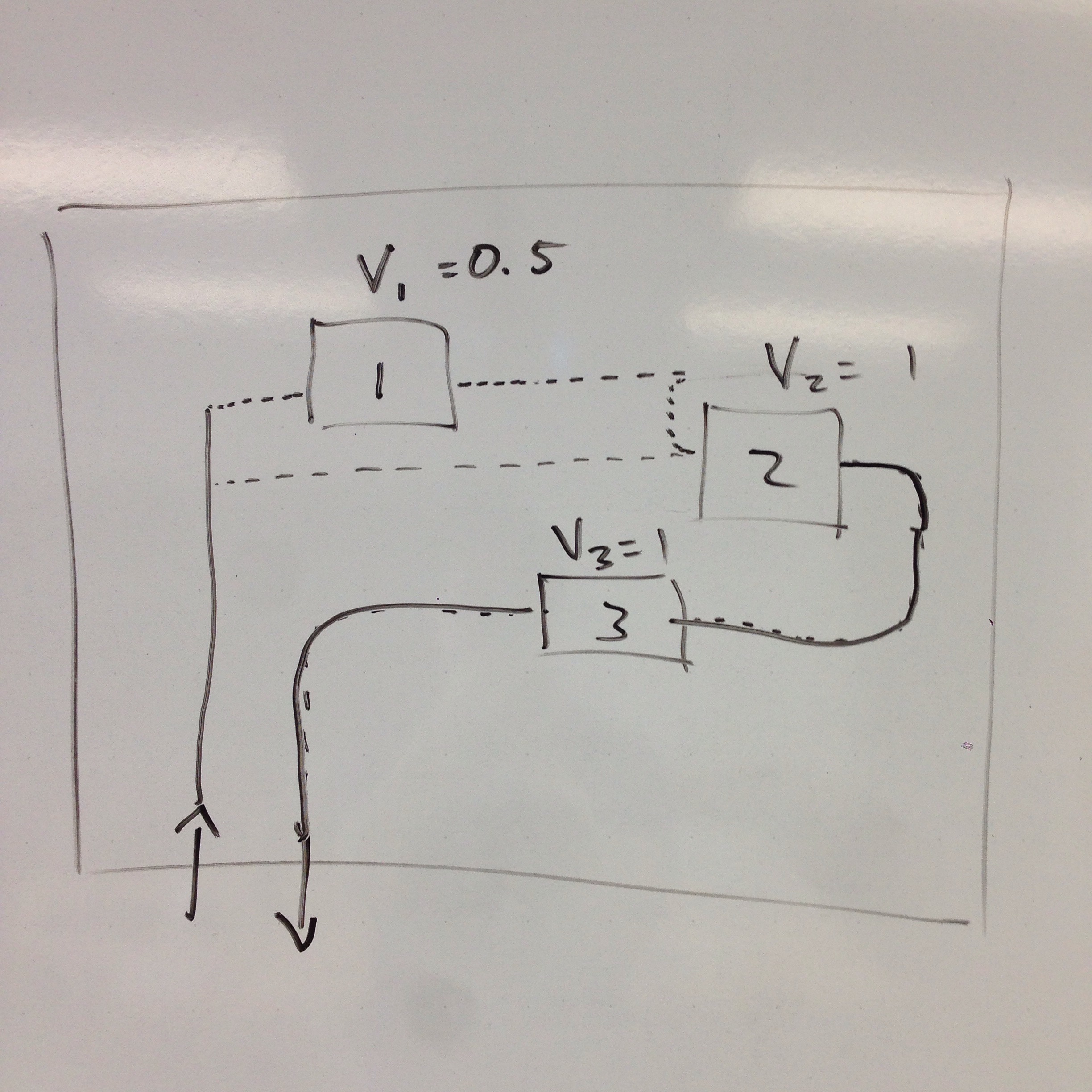
Compared with DRAM, phase change memory (PCM) can provides higher capacity, persistence, and significantly lower read and storage energy (all at the cost of higher read latency and lower write endurance).  In order to take advantage of both technologies, several heterogeneous memory architectures, which incorporate both DRAM and PCM, have been proposed.  One such proposal places the memories side-by-side in the memory hierarchy, and assigns each page to one of the memories.  I propose that the VMIN algorithm described above can be modified to minimize total access latency for a given pair of average (DRAM, PCM) memory usage.

Using the following variables:

• n: Length of program’s memory access trace
• F: Miss/fault ratio (fraction of accesses that are misses to both DRAM and PCM)
• H_DRAM: Fraction of accesses that are hits to DRAM
• H_PCM: Fraction of accesses that are hits to PCM
• R_F: Cost of a miss/fault (miss latency)
• R_H,DRAM: Cost of a hit to DRAM
• R_H,PCM: Cost of a hit to PCM
• M_DRAM: Average amount of space used in DRAM
• M_PCM: Average amount of space used in PCM
• U_DRAM: Cost (“rent”) to keep one item in DRAM for one unit of time
• U_PCM: Cost (“rent”) to keep one item in PCM for one unit of time
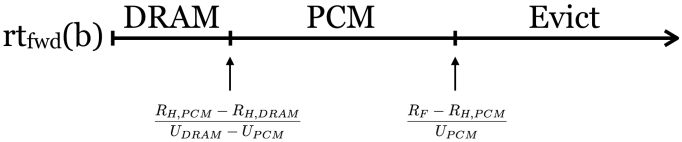
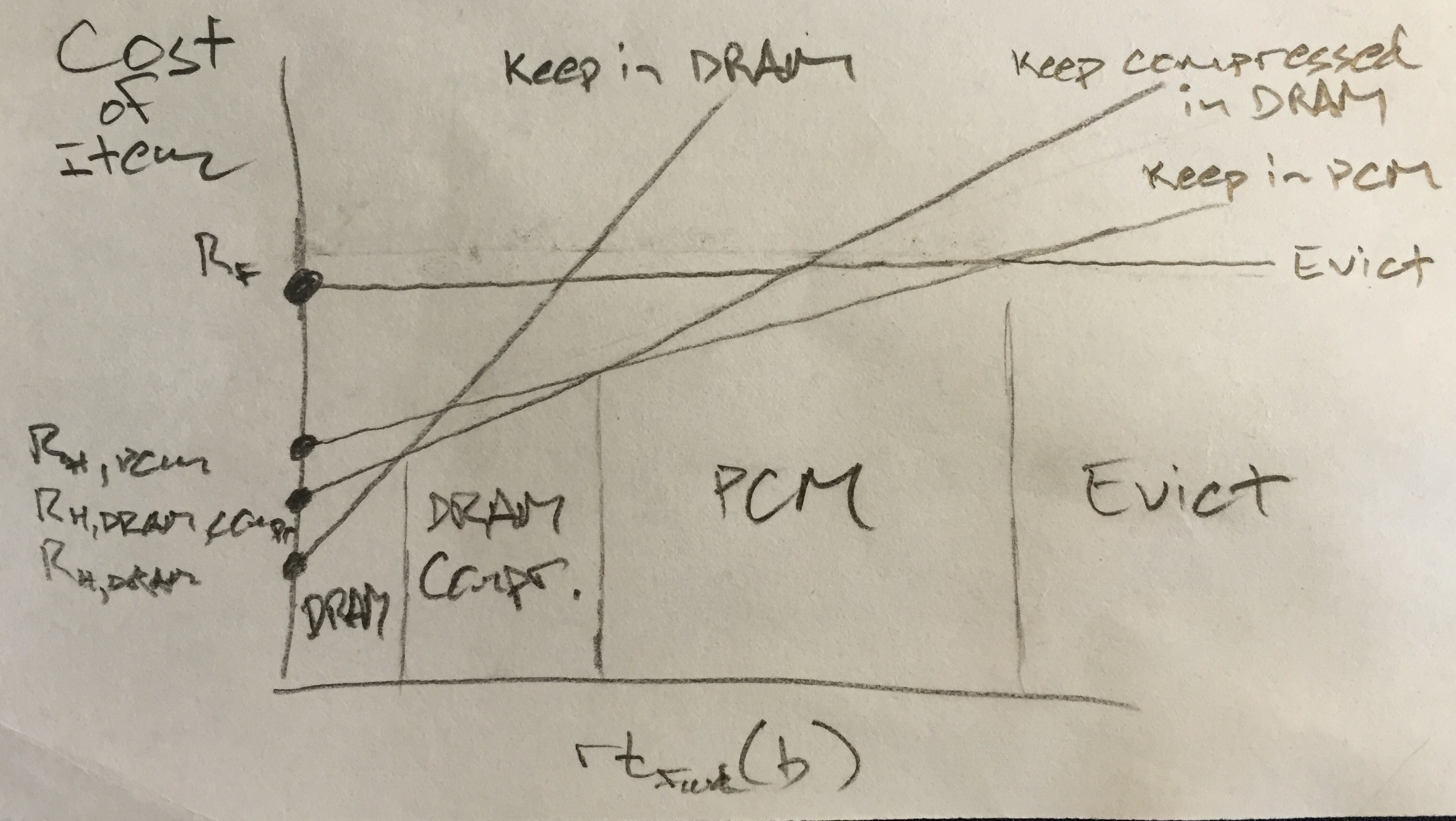
• rt_fwd(b): The forward reuse time of the currently accessed item, b

Define the cost of running a program as C = nFR_F + nH_DRAMR_H,DRAM + nH_PCMR_H,PCM + nM_DRAMU_DRAM + nM_PCMU_PCM, where we are now counting the cost of a hit to each DRAM and PCM, since the hit latencies differ.  If at each access we have the choice to store the datum in DRAM, PCM, or neither, until the next access to the same datum, the cost of each access b is rt_fwd(b) * U_DRAM + R_H,DRAM if kept in DRAM until its next access, rt_fwd(b) * U_PCM + R_H,PCM if kept in PCM until its next access, and R_F if it is not kept in memory.  At each access, the memory controller should make the decision with the minimal cost.

Of course, by minimizing the cost associated with every access, we minimize the total cost of running the program.  The hit and miss costs are determined by the architecture, while the hit and miss ratios, and the DRAM and PCM memory usages are determined by the rents (U_DRAM and U_PCM, respectively).  The only tunable parameters then are the rents, which determine the memory usage for each DRAM and PCM. The following figure (which assumes that U_DRAM is sufficiently larger than U_PCM) illustrates the decision, based on rt_fwd(b):

Update: an alternative diagram, showing the cost of keeping an item in each type of memory vs. the forward reuse distance (now including compressed DRAM):

Since the only free parameters are U_DRAM and U_PCM, this is equivalent to having two separate values of τ, τ_DRAM and τ_PCM in the original VMIN policy.  The WS policy can be adapted by simply choosing a WS parameter for each DRAM and PCM.

If DRAM compression is an option, we can quantify the cost of storing an item in compressed form as rt_fwd(b) * U_DRAM \ [compression_ratio] + R_{H,DRAM_compressed}.

In my last post I talked about the space-time throughput law, and how it can be used to maximize throughput (by minimizing memory space-time per job). This concept is Denning, Kahn and Leroudier argue in their 1976 paper “Optimal Multiprogramming” for the “knee criterion”, which I wrote about on April 30, 2015. In summary, a program’s lifetime curve plots the mean time between misses (called the lifetime) against its mean memory usage. The knee criterion recommends operating a program at the knee of its lifetime curve.

The Knee Criterion

The argument in “Optimal Multiprogramming” is as follows. Let “virtual time” be counted in memory accesses. Using the following variables…

• K:  The number of page faults during a program’s execution
• x:  Its mean memory usage
• G(x):  Its lifetime function (or mean virtual time between faults, for a given x)
• D:  The fault delay (in virtual time – i.e., how many accesses could have been satisfied if it weren’t for the miss.)

The program executes in time approximately KG(x) + KD, and totals KG(x) references. The memory space-time per reference is can then be written

The knee of the lifetime curve (see Fig. 4 below) minimizes x/G(x), and thus “the component of memory space-time due to paging”.

I have one question about this argument though: Why are we only concerned with the one component [x/G(x)]*D?  The space-time throughput law implies that we should minimize the space-time per job, not the component of space-time per job due to paging, right?  This argument doesn’t make intuitive sense to me.

Processor-Utilization and Memory

Consider a system with multiple CPUs sharing cache, and a pool of jobs to be run. The goal is to maximize the job throughput, which can be done by maximizing the fraction of processor time spent active and not waiting for misses. For each processor i, let’s call this quantity the processor-memory utilization:

where Di is now the average delay due to a miss for the program on processor i. Modern processors amortize the effects of LRU cache misses (or what would be LRU cache misses) using optimizations such as superscalar, out-of-order execution, load/store forwarding and prefetching, but I am making the assumption that a program’s total run time can be expressed in the form KG + KD, where K is the number of cache misses, G is the lifetime (inter-miss time), and D is a correlation coefficient, all based on a given caching policy.

Note that the utilization here now measures accesses per time, where in the above argument for the knee criterion, space-time per access was used. Utilization per space is the multiplicative inverse of space-time per access. Following the policy of maximizing space-time per job, we could maximize utilization per space, but with a fixed total memory size, that is equivalent to simply maximize utilization.

When the processor is idle (no job is assigned to it) its processor-memory utilization is taken to be zero. Now, if we define the system processor-memory utilization as the sum of that quantity for each CPU:

If the miss ratio is the multiplicative inverse of the lifetime function, then this becomes

where, as before, the utilization of processor i is taken to be zero when no job is assigned to the processor.

Up to this point, we haven’t needed to mention what caching policy we are using. However, the miss ratio of each program is dependent on that. For global LRU, the miss ratio can be calculated with natural partition theory. For partitioned LRU, it can be calculated with HOTL. For WS, the lifetime (inter-miss time) function may need to be monitored during program execution.

In queuing theory, there are several theorems, e.g., that the mean service time U equals the product of the arrival rate A and the mean service time S (U = AS).  In queuing theory, this is understood to be true when time is sufficiently large (in the limit as time goes to infinity).  In the 70’s, Jeff Buzen and Peter Denning demonstrated that several “limit” theorems from queueing theory were true not just for infinite time, but also for any finite time T.  They called the new results “operational laws”, under the umbrella term of “operational analysis”.

Proved in Buzen’s 1976 paper “Fundamental Operational Laws of Computer System Performance”, the space-time throughput law states that throughput X of a system is equal to the time-average of memory space M used divided by the total space-time used per job Y.  That is, X = M/Y.  An intuitive derivation (though not a proof) can be stated as follows: the space-time is MT, and the number of jobs completed is XT, so the space-time per job is Y = MT/XT = M/X.

While it may at first seem mild-mannered, this law has a powerful implication.  When memory M is fixed, throughput can be maximized by minimizing the space-time per job.  This means that a set of processes sharing a memory will enjoy maximum throughput if each one minimizes its space-time.  One strategy for doing this is to assign some cost (or “rent”) for a process’s use of memory space.  Prieve and Fabry do this in their 1976 paper “VMIN–An Optimal Variable-Space Page Replacement Algorithm”.  Given some memory cost per unit per time U, and some cost of a page fault R, the cost of running a process to completion is C = nFR + nMU, where n is the number of memory accesses made, M is the average amount of memory in use on a memory access, and F is the page fault rate (faults per access).

Optimal Multiprogramming
Denning, Kahn, Leroudier, Potier, Suri

In this paper, the authors give three memory-based techniques for maximizing throughput in a multiprogrammed system. “n” is the number of processes sharing processor time, or the “load”, and T(n) is the throughput.

First they develop a model for their system.

a_i is the request rate for station i, and b_i is the service completion rate for station i. q_i is the fraction of departures from the processor that go to station i (q_0 is a departure). Station 1 is the paging device, so the page swap time is 1/b_1.

A couple of relationships:

b_0 = a_0 + … + a_m (there are m stations)

L(n) = 1/a_1 (system lifetime is average time between page faults)

q_i = a_i/b_0 (by definition, access rate at i / completion rate of processor)

T_i(n) is the throughput at station i. T(n) = T_0*q_0 (output rate of processor * fraction of that that leaves system).

“Three Load Control Rules”
————————–
(1) The Knee Criterion
– Throughput is maximized when memory space-time per job is minimized. In a lifetime curve, the knee is the point that minimizes the memory space-time due to paging. This can be done by managing the memory so that the sum of working set sizes is near the knee.

(2) L = S Criterion
– L is system lifetime, and S is swap time. When the lifetime (time between page faults) is greater than the swap time (time to satisfy a page fault), this prevents queueing at the paging device, which would make it a bottleneck. This rule can be enforced by management of the memory, or by management of the load.

(3) 50% Criterion
– The idea here is to keep the paging device busy between 50% and 60% of the time. This can be enforced by managing the load.

In this paper, the authors show how to adapt the reuse distance metric to account for invalidations and cache sharing. Their additions to the model improve its performance by 70% for per-core caches and 90% for shared caches.

Reuse distance analysis does not traditionally consider associativity, block size or replacement policy. Also, multicore systems have additional complications: “Private caches are typically kept coherent using invalidations”. The second problem is the primary target of this paper.

For example, if one thread writes to a datum between two reuses by another thread, there may be an invalidation, and the second reuse will be a miss even if the reuse distance is short.

Alternatively, a thread may experience a hit on its first access to a datum because another thread brought it into their shared caches.

Models
——

Private Caches with invalidation-based coherence:

* Model uses per-thread reuse distance stacks. A write to any address removes that address from all other stacks containing it.

Shared Caches:

* Use a shared reuse stack.

Hierarchical Structures:

* Combine the two models.

Experiments:

They built reuse distance CDFs for 13 benchmark programs using 3 methods: (1) Simulated cache, (2) model-unaware, (3) model-aware. Results were plotted for 12 of these benchmarks, showing that there is significant difference between those methods. Two tables are presented, showing the percent error of (2) and (3) from (1) for private caches, and for shared and pairwise shared caches.

The results show that the prediction accuracy is significantly higher using the invalidation-based and sharing-aware models.

This paper studies “lifetime functions”, a measure of the time between faults, for LRU and WS page replacement policies, using contrived page access traces based on the working set model. The paper demonstrates that this model is able to reproduce some “known properties of empirical lifetime functions”.

The lifetime is defined as 1/f, where f is the fault rate. It can be thought of as the average virtual time between misses in a program, and expressed as a function of the average space allocation (a.k.a. resident set size) x. For LRU, x = r, the constant amount of space allocated to the program. For WS, the working set replacement algorithm, x the average of r(k) over all references k:

x = 1/k * \sum_{k=1}^K r(k).

Four properties of lifetime functions are defined:

(1) Lifetime functions usually have an S-curve shape.

(2) The WS lifetime is typically higher than the LRU lifetime.

Ideal Estimator:

(a) Resident set is a subset of the current locality set.

(b) At a transition, the resident set contains only pages in both the incoming and outgoing locality sets.

(c) “Page faults occur only for first references to entering pages.””

H: Mean phase duration (“holding time”).

M: Mean number of pages entering, at a transition.

(3) At the knee of the WS lifetime curve, the lifetime is approximately H/M. Intuitively, this is because at the ideal space allocation, H/M is the ratio of time:misses.

(4) There are some (defined) bounds on the difference between the placement of the knees of the lifetime curves for a fixed-space policy and the mean locality size, for Gaussian distributed locality set sizes.

Denning and Kahn go on to describe their program model. There is a macromodel and a micromodel. The macromodel describes how locality sets (working sets) come and go, and the micromodel describes what is done within the locality sets. For the macromodel, they use a semi-Markov model where the working set is the state of the system. They define the parameters of the semi-Markov model: holding time distribution; working set size distribution; and phase transition probabilities, which are only dependent on the phase transitioned to (each column of the transition matrix is consists of all-same numbers).

In the model they used mutually disjoint locality sets.

The Micromodels chosen are:

(1) Cyclic: e.g. abcabcabc…
(2) Sawtooth: e.g. abccbaabccba…
(3) Random: e.g. cabbabcccab…

Results:

Denning and Kahn show results that demonstrate that their program model generates lifetime curves that mimic empirical ones, specifically regarding the four properties of lifetime functions outlined above.

The below photo shows an interpretation of the working set model for memory access behavior.  Each point is a data access belonging to either the “x”, “o” or “star” working set.  Phases of the program are regions where a single working set dominates (shown with brackets).  The ideal choice for working set window size is large enough to encapsulate entire working sets, but small enough to fit within phases.  In this paper, the authors describe the model where working sets overlap, but use a more basic model where working sets do not overlap.

Introduction

————

Profiling repetitive behavior in programs has historically been difficult. “Active profiling” identifies program phases by controlling the input of the program, and monitoring the occurrences of basic blocks in execution.

There are two important definitions:

(1) Phase: “A unit of predictable behavior in that its instances, each of which is a continuous segment of program execution, are similar in some important respect.”

(2) Phase Marker: A basic block that, when executed, is always followed by an instance of the program phase it marks.

The above figure (Figure 2 in the paper) shows the IPC over logical time for GCC compiling a series of identical loops.

Selecting Phase Markers
———————–

The paper presents a 3-step method for identifying phase markers:

(1) The program is given a test input with f identical requests (e.g. in the figure compiling the same loop f times). Basic blocks which execute exactly f times are then selected as potential phase markers. Candidate phase markers whose inter-occurrence distances vary significantly are removed from consideration (because actual phase markers should occur at regular intervals).

(2) Analysis tests whether each remaining candidate occurs g times with other inputs that have g non-identical requests. If not, the candidate is removed from consideration.

(3) In step 3, inner-phases and their phase markers are identified.

Evaluation
———-

They test their system on 3 different programs with repetitive inputs, and show figures with phase markers for each:

(1) GCC: 4 identical functions.

(2) Compress: “A file that is 1% of the size of the reference input in the benchmark suite”. Compress has inherent repetition, because it compresses and decompresses the same input 25 times.

(3) L1: 6 Identical Expressions.

(4) Parser: 6 copies of a difficult-to-parse sentence.

(5) Vortex: A database and 3 iterations of lookups.

Uses of Behavior Phases
———————–

Garbage Collection: A behavior phase “often represents a memory usage cycle, in which temporary data are allocated in early parts of a phase and are dead by the end of the phase”. If garbage collection is run at the end of the phase, there is likely to be a higher fraction of garbage. Shen et al. implemented “preventive” garbage collection and applied it to the Lisp interpreter L1. (The standard “reactive” type of GC collects when the heap is full). Their testing results showed that preventive GC can result in faster execution times than reactive GC. However, in the test they showed, not using GC was faster than either of the GC options, so I’m not sure what to make of their result.

Memory Leak Detection: “If a site allocates only phase-local objects during profiling, and if not all its objects are freed at the end a phase, it is likely that the remaining objects are memory leaks.” This observation can be used to give programmers recourse to find memory leaks. Additionally, phase-local objects that are not freed by the end of the phase can be placed on the same virtual memory page. If not used, they will just go to disk, and not clog up memory.

Intro

“Algorithm analysis can answer questions about running time of a standalone process, but it cannot answer questions about the performance of a system of processes competing for resources.” This is because things like storage access, i/o, and internet connections can cause delays that are difficult to predict. Queueing theory offers a way to describe (and predict) the time costs associated with such delays.

Queueing Theory Meets Computer Science

In 1909, A. K. Erlang found that the inter-arrival times for phone calls were distributed so that the probability of an inter-arrival time exceeding t decayed exponentially:

P(T>t) = exp(-λt),

with 1/λ the average time between calls. He also found that the length of phone calls were distributed the same way:

P(T>t) = exp(-μt).

Erlang employed Markov Chains (with the number of current calls as the state) to predict the probability of losing a call.

Capacity planning describes how to keep queues from getting too large, in order to prevent delays, and manage response time.

Kleinrock (1964) used capacity planning to predict delays on communication networks.

Buzen and Denning discovered that the assumption of flow balance (#arrivals = #completions) led to same equations as stochastic equilibrium.

Server independence: output rate of a server depends only on its local queue lengths, not on that of any other servers.

Conclusion: “traditional assumptions of queueing theory can be replaced by… flow balance and server independence and still yield the same formulas”.
Calculation and Prediction with Models

Operation Laws

U: Utilization (busy time / time)
S: Mean service time (busy time / jobs)
X: Completion rate (jobs / time)
Q: Mean queue length (jobs)
R: Mean response time for a job (time)

Utilization Law: U = S * X
Little’s Law: Q = R * X
Forced Flow Law: Xi = Vi * X
Response Time Law: R = N/X – Z

Denning gives the example of a wine cellar to demonstrate the principle of Little’s law.  If a restaurant owner would like their wine to be aged R = 10 years, and they sell X = 7,300 bottles per year, the owner should build a wine seller with a Q = R * X = 73,000 bottle capacity.

Balance Equation

λ(n): Arrival rate when system is in state n.
μ(n): Completion rate when system is in state n.
p(n): Fraction of time system is in state n.

Balance Equation: For a system of states {0, 1, … n}, the balance equation is λ(n-1)p(n-1) = μ(n)p(n)

    ATM:

p(n) = p(n-1)λ/μ

Probability of dropping telephone calls:

λ: Arrival Rate
1/μ: Average Call Duration
nμ: Departure Rate

p(n) = p(n-1)λ/(nμ)

Probability of dropping a call is p(N+1) where N is the capacity.

Computing with Models (Multi-Server Models)

In 1973, Jeff Buzen discovered “Mean Value Analysis”, a way to calculate in O(#users * #servers) time the server response times, system response time, system throughput, and server queue lengths. The model is extended from the principles of the operation laws.

This paper develops a method for predicting cycles per instruction (CPI) for two programs that are sharing cache. The method takes phase behavior into account, and is demonstrated to be extensible to larger co-run groups as well.

They “show that CPI and bandwidth can vary significantly across runs of the same set of co-running programs.”
– Because “different phases have varying sensitivities to contention for the shared cache.”

– E.g. for astar/lakes and bwaves corun, slowdown of astar is 1%-17% depending on phase overlapping.

– Brute-force measurement of co-run performance distributions would take too much time. They can do it way faster by using solo-run measurements.

Tools

(1) A cache sharing model from Sandberg et al. “Efficient Techniques for Predicting Cache Sharing and Throughput”. The model only works on phase-less programs, so they “slice” the programs by phases and predict performance based on them.

(2) Cache Pirating: Tests misses, hits and cycles for program on any size cache by running it with “small cache intensive stress application” and changing the stress application’s footprint.

(3) Phase Detection: They use the online “ScarPhase” library to detect and classify phases. It has only 2% overhead and is hardware-independent, so better than just doing phases based on CPI because that is hardware dependent.

Cache Sharing Models

When sharing cache, each application affects the other’s execution rate.

(1) Window-Based: Samples with different windows overlapping between programs. The model needs to be applied to each pair.

(2) Dynamic-Window: Merges all windows that are in a single phase.

(3) Phase-Based: Merges all data within a single phase (even when the phase is repeated as in A1 B1 A2 B2). This one is by far the fastest, and just about as good as others.

Evaluation

They compare overhead and accuracy of predictions vs. exhaustive testing. The phase-based approach is an average of 213x faster and has an average of 0.41% error. But the error is bigger for applications with lots of phase behavior (e.g. astar and bwaves gives 6.3% error).

SPEC CPU2006 benchmarks with single, dual, few, and multi-phase behavior were used.

They show accuracy of predictions with cumulative density function (CDF) plots of target-application slowdown for each program pair (target, interference) over 100 trial runs. Both predicted slowdown and actual slowdowns are plotted, and they do reasonably well. One interesting point is that when the interference program has strong phases, and the target program is short, it might run entirely during one phase of the interference program. This is best shown in Figure 5(j, n, r).

Sources of Error

(1) Cache Pirating: Cache pirating relies on the assumption that the stress application can keep its working set in the cache, but pressure from the target application sometimes confounds this.

(2) Bandwidth: Not incorporated into their model because it requires oracle information. But they do demonstrate (using oracle information) that bandwidth constraints are indeed a source of error.

This paper outlines a technique for identifying locality “phases” in a program’s memory access trace using a multi-phase process:

(1) Reuse Distance Analysis with Variable-Distance Sampling

Variable-Distance Sampling allows a reuse distance histogram to be constructed without taking ever single reuse into account. Firstly, only long reuse distances (above the “qualification threshold”) are considered. Two other thresholds are also used: the “temporal threshold”, and the “spatial threshold” (time since last use, and memory address distance). Secondly, as the data trace is analyzed, the thresholds are changed to ensure that some target number of samples is taken.

(2) Wavelet Filtering

Wavelet decomposition is very similar to a Fourier Transform. It approximates/compresses a signal in terms of orthogonal functions on some domain. Shen et al. use a “Discrete Wavelet Transform (DWT)” to represent the reuse distance over the time domain.

At each time (access), the access is removed if its 1st order coefficient is below a threshold (but I don’t understand why).

(3) Optimal Phase Partitioning

Phase partitioning is optimized for two things: maximizing the number of data accesses in a phase, and ensuring that there are multiple multiple accesses to the same datum. Each data point in the DWT of the reuse distance trace is treated as a node in a DAG. The edge weights are based on the number of data recurrences (of other data) between those two access-nodes. Phases are then partitioned using shortest-path analysis, so that the “distance” (sum of weights) between phase boundaries is minimized (I’m not positive I understand that correctly). The point of this is to eliminates spatial redundany.

(4) Phase Hierarchy

A linear-time, linear-space algorithm called SEQUITUR is used to compress the string of memory accesses into a regular grammar.
Phase markers are then inserted into the program.

EXPERIMENTS

Miss rate consistency across runs:
Simulations (Fig. 3).
On IBM Power 4 Machine (Fig. 4).

Adaptive Cache Resizing
During execution, the cache can be resized to suit the working set size without increasing the miss rate. This saves energy. Fig. 6 shows the resulting cache size changes for various methods, including for phases. Overal, phase predictions outperforms the competitors.

Memory Remapping
Phase based memory remapping (by affinity) increased a couple of benchmarks (Mesh and Swim) by ~4% and ~35%.