Intro

“Algorithm analysis can answer questions about running time of a standalone process, but it cannot answer questions about the performance of a system of processes competing for resources.” This is because things like storage access, i/o, and internet connections can cause delays that are difficult to predict. Queueing theory offers a way to describe (and predict) the time costs associated with such delays.

Queueing Theory Meets Computer Science

In 1909, A. K. Erlang found that the inter-arrival times for phone calls were distributed so that the probability of an inter-arrival time exceeding t decayed exponentially:

P(T>t) = exp(-λt),

with 1/λ the average time between calls. He also found that the length of phone calls were distributed the same way:

P(T>t) = exp(-μt).

Erlang employed Markov Chains (with the number of current calls as the state) to predict the probability of losing a call.

Capacity planning describes how to keep queues from getting too large, in order to prevent delays, and manage response time.

Kleinrock (1964) used capacity planning to predict delays on communication networks.

Buzen and Denning discovered that the assumption of flow balance (#arrivals = #completions) led to same equations as stochastic equilibrium.

Server independence: output rate of a server depends only on its local queue lengths, not on that of any other servers.

Conclusion: “traditional assumptions of queueing theory can be replaced by… flow balance and server independence and still yield the same formulas”.
Calculation and Prediction with Models

Operation Laws

U: Utilization (busy time / time)
S: Mean service time (busy time / jobs)
X: Completion rate (jobs / time)
Q: Mean queue length (jobs)
R: Mean response time for a job (time)

Utilization Law: U = S * X
Little’s Law: Q = R * X
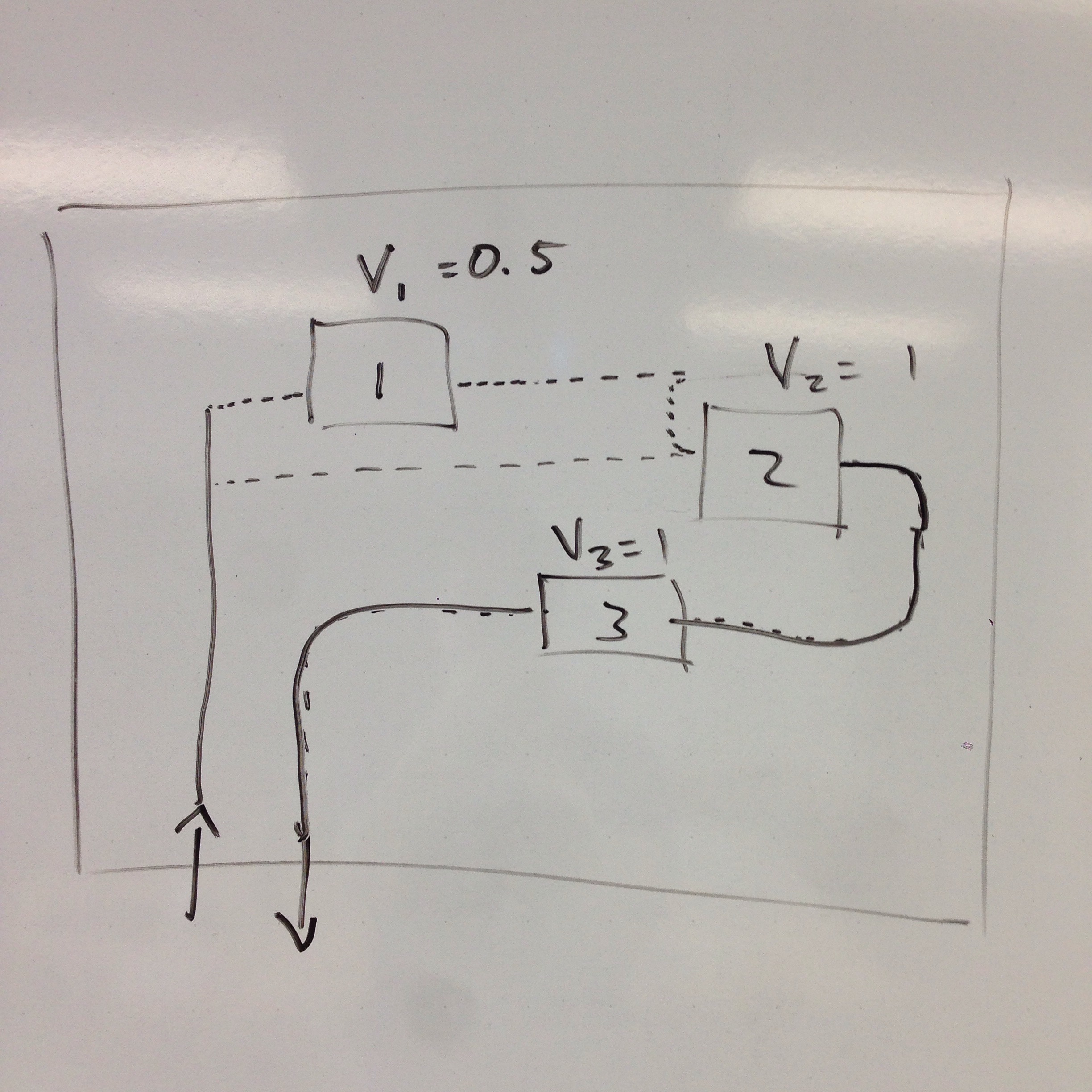
Forced Flow Law: Xi = Vi * X
Response Time Law: R = N/X – Z

Denning gives the example of a wine cellar to demonstrate the principle of Little’s law.  If a restaurant owner would like their wine to be aged R = 10 years, and they sell X = 7,300 bottles per year, the owner should build a wine seller with a Q = R * X = 73,000 bottle capacity.

Balance Equation

λ(n): Arrival rate when system is in state n.
μ(n): Completion rate when system is in state n.
p(n): Fraction of time system is in state n.

Balance Equation: For a system of states {0, 1, … n}, the balance equation is λ(n-1)p(n-1) = μ(n)p(n)

    ATM:

p(n) = p(n-1)λ/μ

Probability of dropping telephone calls:

λ: Arrival Rate
1/μ: Average Call Duration
nμ: Departure Rate

p(n) = p(n-1)λ/(nμ)

Probability of dropping a call is p(N+1) where N is the capacity.

Computing with Models (Multi-Server Models)

In 1973, Jeff Buzen discovered “Mean Value Analysis”, a way to calculate in O(#users * #servers) time the server response times, system response time, system throughput, and server queue lengths. The model is extended from the principles of the operation laws.

Seongbeom Kim, Dhruba Chandra and Yan Solihin

While programs running together, fairness become an important metric beyond throughput. In this paper, authors propose 1) a definition for fairness and 5 possible metrics.  2) 2 algorithms to improve the metrics through cache partition.

According to simulation experiments, authors show that 1) 2 of 5 metrics are not strong correlated to their definition of fairness, 2)LRU or Pseudo-LRU is not fair, 3) Improving fairness usually equal to improving throughput and 4)their cache partition algorithms improve fairness by a factor of 4X while increasing throughput by 15% on average.

More specifically, authors define ideal fairness to be

Where denotes execution time of program i while co-running and for solo-run. Then authors quantitive fairness to be

However, execution time is difficult to measure because of the lack of reference points in the execution. Thus 5 possible metrics are proposed in section 2.3. According to the correlation between these 5 metrics and fairness, turns out 2 metrics are not strong related to fairness and others are sufficient enough. At last authors selected the most correlated metric as following:

After metric is decided, authors proposed 2 algorithms to optimize fairness statically or dynamically. Both of them need additional hardware counter or functionalities. In brief, the static algorithm partition cache before programs running according to stack analysis results, which is gained through profiling. And the dynamic algorithm sampling programs periodically and adjust partition according to measures of sampling phase.

In evaluation, 18 2-programs pairs are tested, the 13 programs come from SPEC2K. A simulator is used with additional hardware counter and functionalities implemented.

Metric correlation is evaluated firstly. They figure out average correlation for all metrics and based on that, they select the best metric which has 94% correlation with fairness.

Then according to comparing between LRU and static partition, LRU produce very unfair sharing in 15 of 18 pairs, and in 3 pairs, LRU is better on fairness. Only in 1 pair, LRU gains better throughput.

The results for dynamic partition is similar. Even though Pseudo-LRU is slightly better than LRU on both throughput and fairness, but it still worse than dynamic partition with only 1 exception, in which PLRU is almost ideal.

Question:

1) For dynamic algorithm, why do not test M0 directly.

2) Not all pairs are tested(18/78)

Andreas Sembrant and etc. proposed a phase-aware model to calculate an application’s miss ratio more efficiently. They combine online phase detection and phase guided profiling to reduce overhead and increase the  accuracy.

The StatCache which proposed by Berg and Hagersten is a low overhead statistical model. It can estimate miss ratio for caches of arbitrary size. But this model only report the average miss ratio which may not fully expose the application’s features. The miss ratio R can be calculated by the following function:

R * N = h₁ f(1*R) + h₂ f(2*R) + h₃ f(3*R) + …

N = h₁  + h₂ + h₃ + …

f(n) = 1 – (1-1/L)ⁿ

N is the number of reuse distance samples, f(n) is the function that indicate the probability that a cache line has been evicted from the cache when it was in the cache n cache misses ago. L is the number of cache lines in the cache.

One simple solution is that divide the program into window and sampling for each window to handle program phases. But the overhead will be significantly increase to capture the short application phases. To avoid this overhead, phase detecting algorithms are used to divide the program into different phases, sampling each phase once is enough and the subsequent instances of the same phase can use the same profiled data.

Based on this thinking, They proposed the ScarPhase (Sample-based Classification and analysis for Runtime Phases). They group the reuse distance of the program by phases and than apply the StatCache model to calculate the miss ratio for each group. They use ScarPhase library to detect and classify phases base on the application’s execution history.

Also they found that variations can also happen inside phases and classified them into four types: No variations, Transition variations, Periodic variations and Instance variations.

(1)No variations mean little changes happened inside the phase, so only a small part of each phase needs to be profiled.

(2)Transition variations mean the behavior slowly changes form one phase to another. So the transition should be divided into windows from the start to the end. More windows to profile, more accuracy we gain.

(3)Periodic variations mean the behavior changes rapidly and periodically.

(4)Instance variations mean the same phase operating on different data may have different miss ratio.

Compared with StatCache model, the ScarPhase increases accuracy by 39% and efficiency by 600%.

In this chapter of the book, some techniques in optimization of loop-based programs’ prallelism and locality are discussed. It starts with an introduction of the basic concepts: the affine access pattern of the data references. Three types of spaces: the iteration space, the data space and the processor space. The essential problem of optimization is to increasing loop’s parallelism and locality, by building multidimensional spaces and affine mappings between these spaces and transforming the loops accordingly.

The chapter is divided into two parts: first, introducing the model of the loops and second, introducing the techniques of

optimization.

Start from the first part. First, how the loop is structured. The loop nests are structured as a multidimensional vector space. The loop bounnds and accesses are represented as set of affine constraints, which can be abstracted as a matrix-vector multiplication form. Symbolic constants (or parameters) are introduced and can be modeled. Next, only the affine accesses can be modeled and they represent many programs in real world. Third, data reuse is categorized into two types: self reuses and group reuses. Self reuse means the reuse is from the same ‘static’ access, while group reuse means the reuse is from different ‘static’ access. The self reuses bring huge savings on memory accesses and the amount of savings can be calculated as the rank of the coefficient matrix in the access. Group reuses are actually a more interesting case, but its analysis limited to accesses whose coefficient matrix are the same. The fourth, representing data dependence. Three types of dependencs are first introduced: true dependence, anti dependence, and output dependence. Integer linear programming is a general solution of finding dependences, but it is an NP-complete problem. There are three parts of solving the integer linear programming problem. First, check the existence of the solution, by using Greatest Common Divisor (GCD) test. Second, try a set of simple heuristics to handle the large amount of inequalities. If the heuristics fail, try integer programming solvers using branch-and-bound.

The second part of the chapter is optimization based on the first part. Three sections are used to cover parallelization for minimizing synchronization. Three steps are required to perform the parallelization: first, split the computations into many independent units; second, assign the computation units to the processors; third, generate an SPMD program that executes on multiple processors. The first problem that is looked at in the book is the problem of finding parallelism that requires no synchronization. The solution is to respect the constraints of data dependence by assigning the operations that share data on one processor. In practice, software pipelining is used to partition programs that minimizes the synchronization between processors. (need more details on this part)

The last part of optimization is to optimize for locality. Three techniques are introduced in the book for both uniprocessors and multiprocessors. First exploiting temporal locality. It basically schedules computations that share data close enough in execution. This part in the book is rather general, only an example is provided to demonstrate the concept. Second, array contraction. When a sequential execution that operates on one array element at a time serially, the array can be contracted by replacing the intermediate array with a scalar. It reduces the need for data storage, but also reduces the parallelism available. The third, interleave the partitions. Two primitives can be employed to reduce the distances between reuses across different iterations. These two primitives can be repeated. Interleaving inner loops in a parallel loop, known as ‘strip-mining’. It blocks the outer loop and moves the blocked loop inside the inner loop to create more reuses within the blocks. Interleaving statements in a parallel loop. This transformation distributes a ‘stripmined’ loop across the statements. It shortens the distance between one statement within a loop using blocking. It is effective when there is a large loop ‘interferes’ the data reuse of one statement in the loop.

There are other forms of affine transformation, mainly targeting on distributed memory machines, multi-instruction-issue processors and vector/SIMD instructions. Prefetching is also briefly mentioned.

Harold S. Stone, Fellow, IEEE, John Turek, Member, IEEE, and Joel L. Wolf

While improving locality through cache management, one of the most significant problems is determining how close is our approach to the optimal one. For sequential program, we get OPT replacement algorithm. And for co-runed programs, we should have one. This paper tried. Authors figure out a model on analyzing quality of partition, figuring out optimal partition and dynamically close to it.

This paper contributes in 4 aspects:

• Optimally partition cache for 2 programs
• Find a partition which has similar performance as LRU
• Theoretically show LRU is far from optimal for transient data allocation
• Near optimally partition cache for N programs

Optimally partition cache for 2 programs

Authors start modeling with an insight that miss ratio is linear to cache size in log/log scaling. Thus they got a prediction function for miss ratio that MI(x)=aI*x^(bI*log10), where x is cache size assigned to program I, a and b are coefficient which got from profiling.

Since the total misses is TotalMisses=(MI(x)+MD(C-x))*T/2, where C is total size of cache, and they suppose the two programs I and D has same access rates T. Then within an assumption that the miss ratio is convexity according to cache size, they can got minimal point for TotalMisses when derivation equal to 0.

Combined with there miss ratio function, authors got optimal partition size with followed equation: bI*aI*log10*x^(bI*log10-1)-aD*bD*log10*(C-x)^(bD*log10-1)

Find a partition which has similar performance as LRU

To achieve this goal, authors firstly propose a concept named state of cache for 2 programs. A State x of cache means overall miss ratio without partition is equivalent to a partition, which  assign x cache for program I and C-x for program D. And S(x) is possibility function of state x appears.

Since the possibility of stat x transforms to  x+1 should be equal to the possibility of x+1 to x, then they have such equation that S(x)MI(x)=S(x+1)MD(C-x-1). According to the monotonic property of MI and MD, S(x) is unimodal.

Finally, for the most possible stat x’, authors showed it is close to optimal partition.

LRU is far from optimal for transient data allocation

With derivation of stats according to time, authors shows LRU needs time to achieve state x’, which is the most possible state as well as the state near to optimal partition.

Since derivation of state x can be represent as dx/dt = Rate of increasing x – Rate of decreasing x,  which is essentially equal to MI(x) – MD(C-x). This derivation shows velocity and time for LRU to achieve a near optimal partition state, and also shows when time is short enough, LRU cannot perform close to optimal.

Near optimally partition cache for N programs

With the assumption that miss ratio function is convexity, authors propose a greedy algorithm to achieve a near optimal solution according to the insight of the first section, which is optimal is achieved when the sum of derivation of miss ratio equal to 0. Thus they employ followed algorithm keep the sum as close to 0 as possible:

Let Ci to be cache size of partition i

Initialization: set C1=C2=…=CN=0

Induction step : Find the most benefit programs i, which would reduce the most cache misses with extra 1 cache block

let Ci=Ci+1, and keep other partition does not change, goto step 2 until sum of partition size equal to C

Why writing efficient parallel code is difficult?

The reason is that  the performance of a parallel program is dependent on many factors. Mark Edward Crovella who was awarded Phd degree by URCS in 1994 divided the factors into two groups: external factors and internal factors.

External factors are the aspects of the program’s run-time environment which is not specified in the parallel program:

1: the number of processors used to run the program

2: the size of the input data set

3: the structure of the input data set (sparseness of a matrix)

4: the problem definition (a program can solve multiple variations of a problem)

5: the machine used to run the program (architecture)

Internal factors are the methods used to parallelize the application. Typical examples of internal factors are:

1: type of parallelism used

2: which code to parallelize

3: synchronization methods

The external factors will determine the choice of internal factors. Programmers should not expect to find one general best structure for parallel program. With these insights, he proposed three techniques to assist rapid development of parallel efficient programs: Predicate profiling, lost cycles analysis and lost cycles modeling.

Predicate profiling:

The standard formula to measure the performance of parallel program is described below. But To(n,p) is not specified which is not so helpful for optimization. Because the reasons cause the overhead are not exposed.  So he decomposed To(n,p) into performance predicates.

  Tp(n,p) = ( To(n,p) + Tc(n) ) / p

Speedup:

S(n,p) = Tc(n) / Tp(n,p)

Efficiency:

E(n,p) = S(n,p) / p = Tc(n) / (p * Tp(n,p)) = Tc(n) / ( To(n,p) + Tc(n) )

p: number of processor

   n: input data size

To(n,p): total overhead in an execution

   Tc(n): non-overhead or “pure” computation

   Tp: the execution time of parallel application

To(n,p) are broke into the synchronization loss, communication loss, workload imbalance, insufficient parallelism, resource contention.

“Workload imbalance(LI): processor cycles spent idling, while unfinished parallel work exists.

Insufficient parallelism(IP): processor cycles spent idling, while no unfinished parallel work exists.

Synchronization Loss(SL): processor cycles spent acquiring a lock, or waiting in a barrier.

Communication Loss(CL): processor cycles spent waiting while data moves through the system.

Resource Contention(RC): processor cycles spent waiting for access to a shared hardware resource.”

Lost cycle analysis and modeling:

In there states, no useful work is down, so they call the time spent in the stats Lost Cycles (LC). So he model each component of To instead of modeling To which will reduce the difficulty in modeling.

To(E) = IP(E) + LI(E) + SL(E) + CL(E) + RC(E)

IP, LI, SL, CL, RC are functions of n and p with parameters. And the parameters are determined by the predicate profiling data. With parameters set down, the components of the  overhead can be exposed which can guide the optimization.

The increasing gap between memory latency and processing power requires a model under which we can decompose
these two. This book discusses models of memory hierarchy that suit this purpose.

The simplistic “external memory model” models the memory hierarchy as an internal fast memory and an external memory. The CPU operates on the internal memory. The external memory can only be accessed using I/Os that move B contiguous words between internal and external memory. The number of these I/O transfers defines the performance of an algorithm under this model, while the CPU performance is defined by the processing work on the internal memory.

In a real memory hierarchy, a hardware cache uses a fixed strategy to decide which blocks are kept in the internal memory, whereas the external memory model gives the programmer full control over the content of the internal memory. This difference will probably not have devastating consequences as prior work has shown that in practice we can even circumvent hardware replacement schemes.

It is important to design algorithms that perform efficiently under this model. A relatively simple example illustrated in the book is implementing a stack. A naive implementation of the stack leads to O(N) transfers between internal and external memory in the worst case, where N is the number of stack operations (push and pop). However, using a buffer of size 2B (B being the block size), we can achieve amortized performance of O(N/B).

The book designs and analyzes efficient algorithms for several other fundamental problems such as sorting, permuting, and matrix multiplication.

The second model is the “cache oblivious model.” Algorithms designed for the external memory model need to know parameters of the memory hierarchy in order to tune performance for specific memories. Cache oblivious algorithms, on the other hand, don’t have any knowledge of the parameters M (cache size) and B (block size). Further, it assumes that the internal memory is ideal (a fully-associative cache with optimal replacement policy).

An example illustrated in the book is the “Van Emde Boas Layout” for binary search on balanced trees.

“Given a complete binary tree, we describe a mapping from the nodes of the tree to positions of an array in memory. Suppose the tree has N items and has height h = log N + 1. Split the tree in the middle, at height h/2. This breaks the tree into a top recursive subtree of height ⌊h/2⌋ and √N several bottom subtrees B_1 , B_2 , …, B_k of height ⌈h/2⌉. There are √N bottom recursive subtrees, each of size √N. The top subtree occupies the top part in the array of allocated nodes, and then the B_i’s are laid out. Every subtree is recursively laid out.”

We now can analyze the number of cache misses for a binary search operation on a tree with a Van Emde Boas layout. If we denote by c(h) the number of cache misses on a tree of height h, we have:

c(h) = 2c(h/2) if h> lg(B)
c(h) <= 2 if h<= lg(B)

Therefore, we have c(h) = h – lg(B), which is lg N – lg B where N is the total number of nodes in the tree.

This paper develops a method for predicting cycles per instruction (CPI) for two programs that are sharing cache. The method takes phase behavior into account, and is demonstrated to be extensible to larger co-run groups as well.

They “show that CPI and bandwidth can vary significantly across runs of the same set of co-running programs.”
– Because “different phases have varying sensitivities to contention for the shared cache.”

– E.g. for astar/lakes and bwaves corun, slowdown of astar is 1%-17% depending on phase overlapping.

– Brute-force measurement of co-run performance distributions would take too much time. They can do it way faster by using solo-run measurements.

Tools

(1) A cache sharing model from Sandberg et al. “Efficient Techniques for Predicting Cache Sharing and Throughput”. The model only works on phase-less programs, so they “slice” the programs by phases and predict performance based on them.

(2) Cache Pirating: Tests misses, hits and cycles for program on any size cache by running it with “small cache intensive stress application” and changing the stress application’s footprint.

(3) Phase Detection: They use the online “ScarPhase” library to detect and classify phases. It has only 2% overhead and is hardware-independent, so better than just doing phases based on CPI because that is hardware dependent.

Cache Sharing Models

When sharing cache, each application affects the other’s execution rate.

(1) Window-Based: Samples with different windows overlapping between programs. The model needs to be applied to each pair.

(2) Dynamic-Window: Merges all windows that are in a single phase.

(3) Phase-Based: Merges all data within a single phase (even when the phase is repeated as in A1 B1 A2 B2). This one is by far the fastest, and just about as good as others.

Evaluation

They compare overhead and accuracy of predictions vs. exhaustive testing. The phase-based approach is an average of 213x faster and has an average of 0.41% error. But the error is bigger for applications with lots of phase behavior (e.g. astar and bwaves gives 6.3% error).

SPEC CPU2006 benchmarks with single, dual, few, and multi-phase behavior were used.

They show accuracy of predictions with cumulative density function (CDF) plots of target-application slowdown for each program pair (target, interference) over 100 trial runs. Both predicted slowdown and actual slowdowns are plotted, and they do reasonably well. One interesting point is that when the interference program has strong phases, and the target program is short, it might run entirely during one phase of the interference program. This is best shown in Figure 5(j, n, r).

Sources of Error

(1) Cache Pirating: Cache pirating relies on the assumption that the stress application can keep its working set in the cache, but pressure from the target application sometimes confounds this.

(2) Bandwidth: Not incorporated into their model because it requires oracle information. But they do demonstrate (using oracle information) that bandwidth constraints are indeed a source of error.

This paper outlines a technique for identifying locality “phases” in a program’s memory access trace using a multi-phase process:

(1) Reuse Distance Analysis with Variable-Distance Sampling

Variable-Distance Sampling allows a reuse distance histogram to be constructed without taking ever single reuse into account. Firstly, only long reuse distances (above the “qualification threshold”) are considered. Two other thresholds are also used: the “temporal threshold”, and the “spatial threshold” (time since last use, and memory address distance). Secondly, as the data trace is analyzed, the thresholds are changed to ensure that some target number of samples is taken.

(2) Wavelet Filtering

Wavelet decomposition is very similar to a Fourier Transform. It approximates/compresses a signal in terms of orthogonal functions on some domain. Shen et al. use a “Discrete Wavelet Transform (DWT)” to represent the reuse distance over the time domain.

At each time (access), the access is removed if its 1st order coefficient is below a threshold (but I don’t understand why).

(3) Optimal Phase Partitioning

Phase partitioning is optimized for two things: maximizing the number of data accesses in a phase, and ensuring that there are multiple multiple accesses to the same datum. Each data point in the DWT of the reuse distance trace is treated as a node in a DAG. The edge weights are based on the number of data recurrences (of other data) between those two access-nodes. Phases are then partitioned using shortest-path analysis, so that the “distance” (sum of weights) between phase boundaries is minimized (I’m not positive I understand that correctly). The point of this is to eliminates spatial redundany.

(4) Phase Hierarchy

A linear-time, linear-space algorithm called SEQUITUR is used to compress the string of memory accesses into a regular grammar.
Phase markers are then inserted into the program.

EXPERIMENTS

Miss rate consistency across runs:
Simulations (Fig. 3).
On IBM Power 4 Machine (Fig. 4).

Adaptive Cache Resizing
During execution, the cache can be resized to suit the working set size without increasing the miss rate. This saves energy. Fig. 6 shows the resulting cache size changes for various methods, including for phases. Overal, phase predictions outperforms the competitors.

Memory Remapping
Phase based memory remapping (by affinity) increased a couple of benchmarks (Mesh and Swim) by ~4% and ~35%.