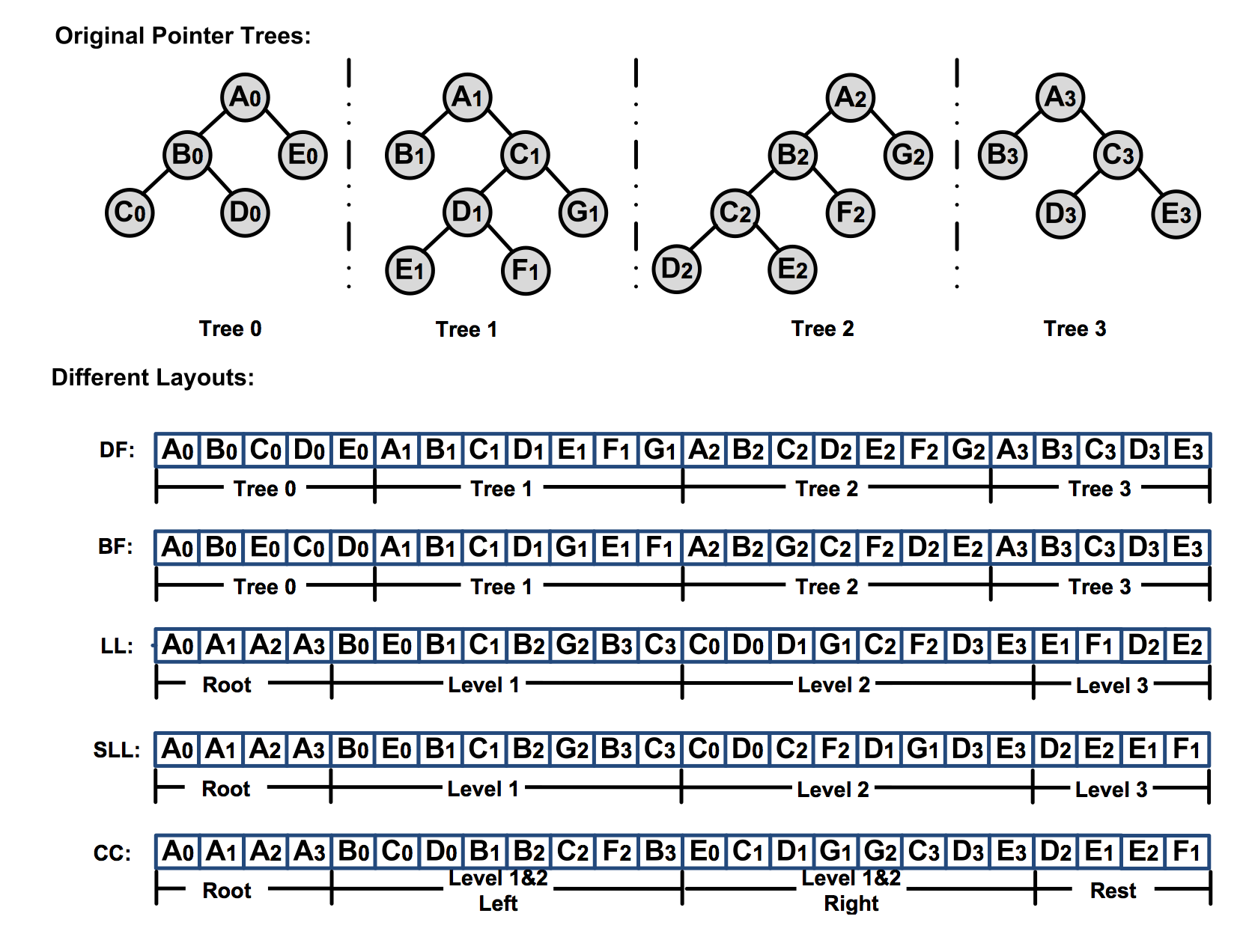
This is the paper that cited 7 of our footprint papers and published in OSDI 2014. The main work is to fast derive workload’s miss ratio curve (MRC). The technique adopted in the paper is a data structure called “counter stack”, which, is essentially a extremely huge matrix of size NxN, where N is the trace length. This data structure is contains the footprint (or working set size) of all windows, (not average window size). From the counter stack, stack distances of references can easily be read. So the challenge this paper addresses is to compress the data structure. The paper talked about some optimizations, which includes, sampling (process every dth reference), pruning (“forget” some windows), using probabilistic cardinality estimator (HyperLogLog) to approximate reuse distances. Using stack counters can be used to query many useful informations, like total data footprint, trace length, miss ratio within a given time period and miss ratio composed from multiple workloads.

So first, what is a stack counter? It is a 2-dimensional matrix. When a new reference is made, a new column is inserted to the right side of the matrix. Each entry C_ij represents the amount of distinct elements in the window (i,j). Therefore this matrix contains footprints of all possible windows of the trace.

Having the matrix, to compute MRC also requires a way to identifies the reuse windows. To do so, two more matrices are needed, \delta x and \delta y.

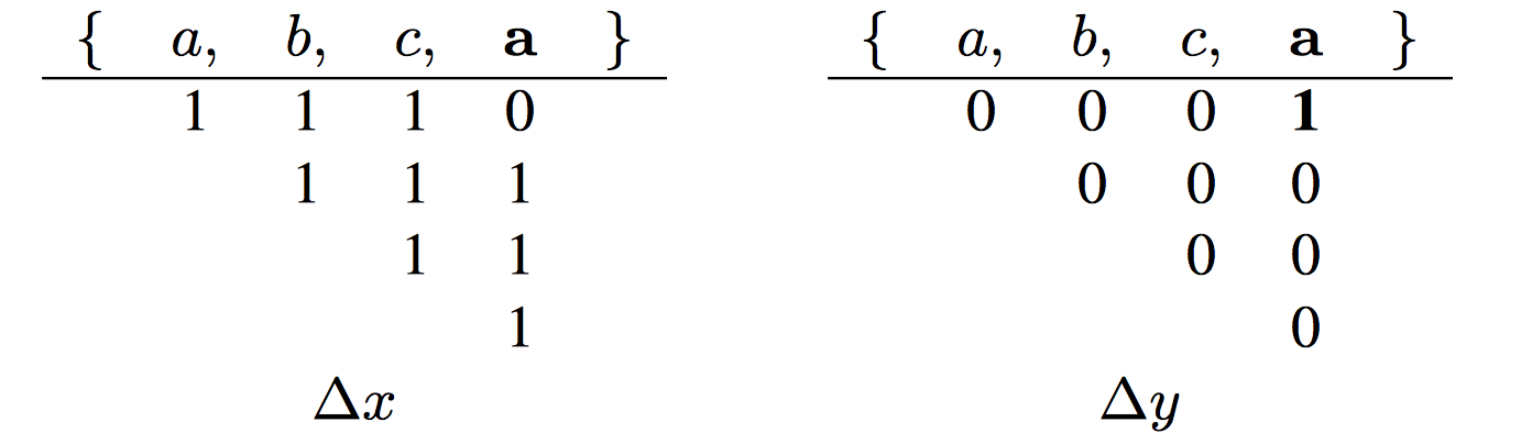
x matrix is the difference of rows of counter stack while y matrix is the difference of rows of x matrix. It seems to me, this differencing operation is “taking directive” in HOTL theory. For the fourth reference in the example trace, the top “1” in the fourth column is at the 1st row, so its last access time is 1.

This is all about counter stack.

To make this data structure practical, there are several approximations presented in the paper.

1. Sampling. A simple approach is to sample every d references. It indicates that the matrix is to be shrinked by a factor of “d”. From the paper, “For large scale workloads with billions of distinct elements, even choosing a very large value of d has negligible impact on the estimated stack distances and MRCs.”

2. Pruning. The observation is that, in x matrix, each rows only contains at most M “1”s, where M is the total footprint. At some point on, the entries in the row will become 0 and remain 0 for the rest of row. Therefore, the paper propose to delete the rows where it has at most M/p different entries than its immediate lower rows. I am not sure how this operation would impact the result and how it can be migrated to our footprint measurement. But, intuitively, this observation, to translate into footprint theory, means larger windows are likely to have most of the data, maintaining large-sized windows at fine granularity is waste.

3. Using probabilistic cardinality estimator. Counter stack needs to counts the amount of data it has seen. It can keep records for all the data using hash table and count the size of the table. It is too expensive. Bloom filter is an option, but “the space would still be prohibitively large”. (I don’t know why…) Therefore, they choose a probabilistic counter or cardinality estimator, called “HyperLogLog“. The memory usage is roughly logarithmic in M with more accurate counters requiring more space.

4. Due to above approximations, the form of \delta x and \delta y matrices is different from shown above. The authors proved a theorem to bound the error by total footprint, trace length and two other parameters.

Counter stack has benefits over stack distance (reuse distance). It has time information. From counter stack, the MRC for any time period can be read by slicing the counter stack. Counter stacks are also composable, because it is essentially “footprint”. However, it still has not solved the problem of interleaving and data sharing. Composing two counter stacks requires alignment beforehand. When data is shared across traces, composition becomes almost impossible.

Above is all technical details about counter stacks. The authors also have some interesting observations about their workloads using counter stack in the paper.

This paper proposed a support for exploiting fine-grained data parallelism (SSE, AVX and GPU) for a set of applications which traverse multiple, irregular data structures (tree, NFA). There are two components in this support: 1. code generation: generating  code that exploits the platform’s support on fine-grained data parallelism in a portable manner. 2. locality optimization: optimize the memory layout to improve inter-thread and intra-thread locality.

The paper is well organized. It first introduced the class of applications (irregular applications with independent traversal) the proposed method targets and challenges in optimizing them (unbalanced workload, divergence, pointer-based traversal). It then specifies the platforms it targets on: x86 system with SSE instructions and NVIDIA GPUs. (SIMD platform). The introduction ends with a list of contributions.

First, code generation and execution. The author developed an immediate language to describe the traversal of the target applications. This immediate language is used to enable portability of the algorithm. A runtime scheduler is responsible to execute the bytecode and perform some necessary dynamic optimization. One specific optimization mentioned in the paper is stream compaction. Stream compaction basically compacts the valid output of a vectorized operation together by “bubbling” the invalid output. This technique, as claimed by the author, can be extended to the GPU platform, with modifications.

Second, optimized data layout. The data layout of irregular data structure is to linearize the data elements in memory. There are two goals here, as clearly specified by the author: 1. co-locating nodes (in the same cache line) that are likely to be accessed concurrently by different threads (inter-thread locality). 2. co-locating threads that are accessed in successive steps by the same thread (intra-thread locality).

Take the traversal of 4 trees as example. There are 5 primitive layouts proposed in the paper. DF and BF correspond to Depth-First and Breath-First, which layout one single tree’s nodes together in memory. LL means level-by-level. It layouts the nodes at the same level (across multiple trees) together in memory. It has better locality for vectorized operations than the first two strategies. SLL is Sorted level-by-level. The author observed that in some cases, during the left children are biased over the right children. Therefore it is beneficial to group the nodes which are left children of their parents together. CC is Cache-Concious. It has an idea that when a parent is traversed, its children may immediately be accessed. Therefore it is beneficial to group parent nodes with child nodes while still maintaining level-by-level layout. These five layouts can be combined to form a hybrid layout, which is, the top x levels use SLL while the rest levels use CC. The value of x is a user-defined parameter, called switching parameter.

The author then analytically described a formula to calculate x for LL-CC hybrid layout and SLL-CC hybrid layout. The model is to minimized cache misses and thus *execution time*. There are assumptions in this model. First, no temporal locality considered, which means one node is traversed exactly once. Second, a complete binary tree. Also, to test whether a certain bias on left/right child exists, sampling is used.

To shortly summarize their evaluation, they observed up to a 12X speedup on one SIMD architecture. They also get as much as 45% speedup over a suboptimal solution.

In this chapter of the book, some techniques in optimization of loop-based programs’ prallelism and locality are discussed. It starts with an introduction of the basic concepts: the affine access pattern of the data references. Three types of spaces: the iteration space, the data space and the processor space. The essential problem of optimization is to increasing loop’s parallelism and locality, by building multidimensional spaces and affine mappings between these spaces and transforming the loops accordingly.

The chapter is divided into two parts: first, introducing the model of the loops and second, introducing the techniques of

optimization.

Start from the first part. First, how the loop is structured. The loop nests are structured as a multidimensional vector space. The loop bounnds and accesses are represented as set of affine constraints, which can be abstracted as a matrix-vector multiplication form. Symbolic constants (or parameters) are introduced and can be modeled. Next, only the affine accesses can be modeled and they represent many programs in real world. Third, data reuse is categorized into two types: self reuses and group reuses. Self reuse means the reuse is from the same ‘static’ access, while group reuse means the reuse is from different ‘static’ access. The self reuses bring huge savings on memory accesses and the amount of savings can be calculated as the rank of the coefficient matrix in the access. Group reuses are actually a more interesting case, but its analysis limited to accesses whose coefficient matrix are the same. The fourth, representing data dependence. Three types of dependencs are first introduced: true dependence, anti dependence, and output dependence. Integer linear programming is a general solution of finding dependences, but it is an NP-complete problem. There are three parts of solving the integer linear programming problem. First, check the existence of the solution, by using Greatest Common Divisor (GCD) test. Second, try a set of simple heuristics to handle the large amount of inequalities. If the heuristics fail, try integer programming solvers using branch-and-bound.

The second part of the chapter is optimization based on the first part. Three sections are used to cover parallelization for minimizing synchronization. Three steps are required to perform the parallelization: first, split the computations into many independent units; second, assign the computation units to the processors; third, generate an SPMD program that executes on multiple processors. The first problem that is looked at in the book is the problem of finding parallelism that requires no synchronization. The solution is to respect the constraints of data dependence by assigning the operations that share data on one processor. In practice, software pipelining is used to partition programs that minimizes the synchronization between processors. (need more details on this part)

The last part of optimization is to optimize for locality. Three techniques are introduced in the book for both uniprocessors and multiprocessors. First exploiting temporal locality. It basically schedules computations that share data close enough in execution. This part in the book is rather general, only an example is provided to demonstrate the concept. Second, array contraction. When a sequential execution that operates on one array element at a time serially, the array can be contracted by replacing the intermediate array with a scalar. It reduces the need for data storage, but also reduces the parallelism available. The third, interleave the partitions. Two primitives can be employed to reduce the distances between reuses across different iterations. These two primitives can be repeated. Interleaving inner loops in a parallel loop, known as ‘strip-mining’. It blocks the outer loop and moves the blocked loop inside the inner loop to create more reuses within the blocks. Interleaving statements in a parallel loop. This transformation distributes a ‘stripmined’ loop across the statements. It shortens the distance between one statement within a loop using blocking. It is effective when there is a large loop ‘interferes’ the data reuse of one statement in the loop.

There are other forms of affine transformation, mainly targeting on distributed memory machines, multi-instruction-issue processors and vector/SIMD instructions. Prefetching is also briefly mentioned.