Peano Curve (from Wikimedia)
Early after, in 1891, Hilbert discovered a simpler variant of the Peano Curve, now known as Hilbert Curve.
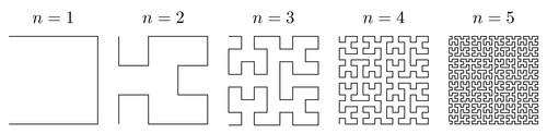
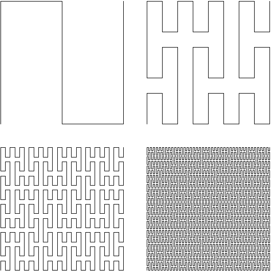
Several Iterations of Hilbert Curve
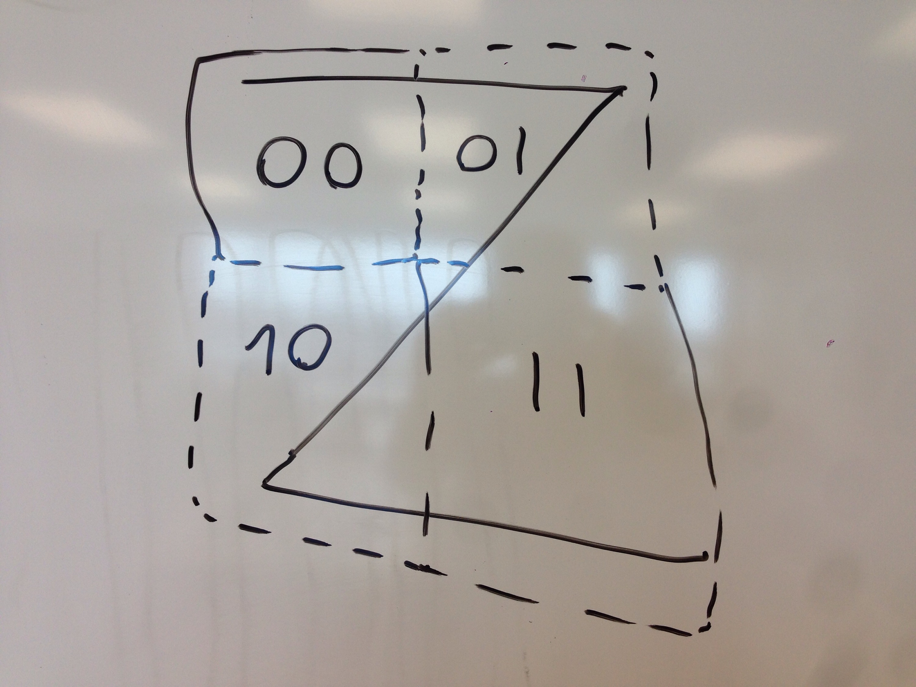
Both Peano and Hilbert curves require rotations. Here’s the Morton (Z-order) curve which doesn’t.
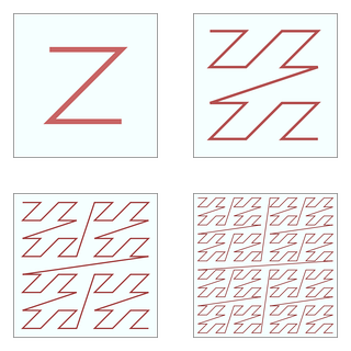
Morton (Z-order) Curve
Space filling curves have the following properties which make them appealing for locality improvement.
- Space-filling: They are continuous functions whose range comes arbitrary close to a given point in the n-dimensional space. Thus they preserve locality at any granularity, regardless of the dimensionality.
- Dimensionality: They exist for all dimensions greater than one.
- Self-similar: They can and are usually defined as non-terminating recurrences.
However, when space-filling curves are used to improve data layout, traversal or indexing of the curve must be efficient. Programming languages often lack support for any indexing other than the canonical one, since they are not as simple to implement. Under the canonical indexing, the relative address of the array element A[i, j] is simply equal to i × n + j, where n is the length of the first dimension of the array. This is efficient to implement in hardware. Furthermore, because this formula is linear, it is easy to compute the address of an element relative to another element in the same row or column. Therefore, in linear traversals of the array, we can avoid the cost of multiplication in the above formula.
Jin and Mellor-Crummey (TMS05) developed a universal turtle algorithm to traverse various space-filling curves using each curve’s movement specification table. They used the same approach to transform the coordinates of a point into its position along the curve (indexing). Interestingly, it turns out that in a Morton curve, the conversion from the canonical index to the Morton index can be carried out in a much more efficient way, by interleaving the bits of the indices.
Research shows that the choice of layout is critical for performance. Frens and Wise designed a QR factorization algorithm specialized for Quadtree layout (a layout very similar to Z-order curve) and showed that not only does it improve reuse but it also improves parallelism due to the reduction in false sharing. Here is a graph illustrating their speedup on a uniprocessor system.
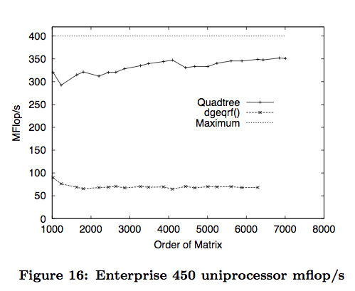
Frens-Wise: PPOPP03
3D view from vismath.eu

In a Morton curve, a jump goes from the upper right corner to the lower left. As a result, the two adjacent points on a Morton curve are not necessarily adjacent in the space being filled. The curve locality may not have any locality in the space. In the reverse relation, some locality in space, e.g. two points straddling the middle point on the left edge of the square, can be far apart on the curve.
In contrast, Peano and Hilbert curves have continuity.
Rahman drew the board photo to show how Morton indexing is done by interleaving the bits of coordinate indices.
A program example can be as follows. We have a 2D matrix, and our program may traverse it by rows or columns. Either of the traditional layout, row- or column-major, does not always provide spatial locality. A space-filling curve layout, e.g. Morton, provides spatial locality (in the linearized layout) as long as the matrix traversal is contiguous in the 2D space, which includes row or column traversals.
Combining loop tiling and space-filing curve data layout (what Wise called non-linear array layout) would mean that data accessed next to each other in time are also adjacent in space.
How do we measure quality of a filling curve, aka, can we compare two curve and tell which one is better?