


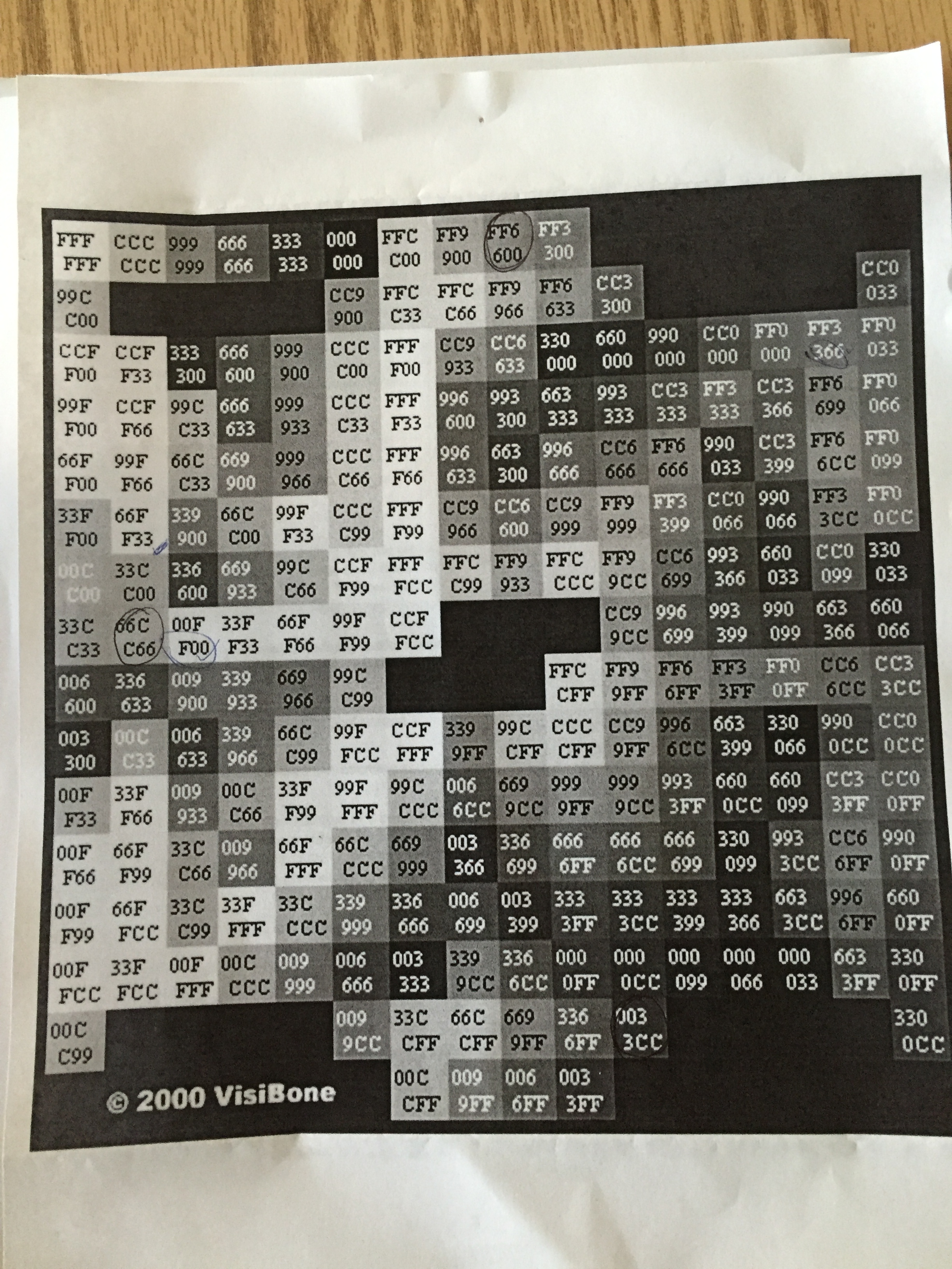
Colored plots/figures may be printed in grayscales which could be difficult to tell.
We can print a color table in grayscale and choose the most distinguishable colors from the printed table. Here is an example:
for three colors, we can use FF6600, 66CC66 and 0033CC.
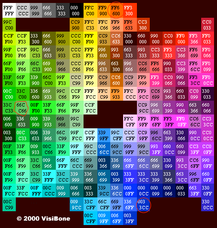
(From http://www.visibone.com)
After the post on computational locality, it is interesting to examine our understanding of physical locality. There is a fascinating storyline in the history of physics.
Einstein is one of the greatest physicists. However, he was always troubled by quantum mechanics whose results, unlike Newton mechanics, are inherently probabilistic rather than deterministic. For example, his quote “God does not play dice with the universe” was actually a direct criticism.
The discovery of two-particle quantum entanglement gave him a chance to formulate his objection precisely. In 1935, Einstein, Boris Podolsky and Nathan Rosen distributed the so-called EPR paradox. They laid out four premises of a physics theory:
[Greenberger et al. 1990] state in EPR’s words.
For a two-particle entanglement, the measurement of particle 1 can cause no real change in particle 2. Until the measurement, the states of particles 1 and 2 have no definite values from the theory of quantum mechanics. Therefore, as a theory quantum mechanics is incomplete.
These objections were unresolved (and largely ignored) by physicists in the next fifty years. A series of studies on Bell Inequality were made, but the experimental setups were open to criticism.
In late 1980s, researchers at University of Rochester especially Leonard Mandel, Professor of Physics and Optics, and his students followed on their studies on the quantum properties of light and invented a technique called parametric down-conversion to produce entangled photons.
Daniel Greenberger, while visitingVienna with Anton Zeilinger, found that a perfect correlation among three particles was enough to disprove EPR. Michael Horne, back at Boston, discovered Mandel’s two-particle interference design based on a “folded diamond. ”
The paper by Greenberger et al. was published in 1990. It shows that for 3 or more particle entanglement, the four EPR premises would derive contradictory results. No theory that meets these four premises can explain the perfect correlation in such entanglements. In the proof by Greenberger et al., (Section III, slightly more than 1 page), “the manipulation of an additional degree of freedom is essential to the exhibition of a contradiction.”
The contradiction shows that either locality or reality assumptions do not hold. The combination of the two is now called “local realism.”
Scully et al. wrote that “In an ingenious experiment with [Zhe-Yu] Ou, Leonard utilized polarization entanglement for photon pairs produced in down conversion to achieve a violation of Bell’s inequality (i.e., local realism).”
I first heard about the story from the book by Aczel and taught the 1990 paper in the opening lecture of a graduate seminar in Spring 2005 on Modeling and Improving Large-Scale Program Behavior.
Greenberger, Daniel M., et al. “Bell’s theorem without inequalities.” Am. J. Phys 58.12 (1990): 1131-1143.
ROBERT J. SCULLY, MARLAN O. SCULLY, AND H. JEFF KIMBLE, “Leonard Mandel,” Biographical Memoirs: Volume 87, The National Academies Press (2005)
Zhe-Yu Ou and Leonard Mandel. Violation of Bell’s inequality and classical probability in a two-photon correlation experiment. Phys. Rev. Lett.61(1988):50.
Amir D. Aczel, Entanglement: The Greatest Mystery in Physics. Random House, Inc. (2002)
Here are three sources people can cite for the definition of locality by Peter Denning:
“The tendency for programs to cluster references to subsets of address space for extended periods is called the principle of locality” on page 143 in Peter J. Denning and Craig H. Martell. 2015. Great Principles of Computing. MIT Press
Locality is “the observed tendency of programs to cluster references to small subsets of their pages for extended intervals.” on page 23 in Peter J. Denning. 2005. The locality principle. Communications of ACM 48, 7 (2005), 19–24
Locality is “a pattern of computational behavior in which memory accesses are confined to locality sets for lengthy periods of time.” in an email from Denning, June 26, 2016.
Given the domain name of this site, it is fitting to have the precise definition of the term here.
Locality has been discussed by others.
In their influential paper titled Dynamic Storage Allocation: A Survey and Critical Review [ISMM 1995], Wilson and others wrote “Locality is very poorly understood, however; aside from making a few important general comments, we leave most issues of locality for future research.”
The two workshops, LCPC and CnC, will be held at Hilton Garden Inn in the college town next to University of Rochester river campus (arts, sciences and engineering) and medical school:
Hilton Garden Inn
Rochester/University & Medical Center
30 Celebration Drive
Rochester, New York, 14620, USA
The LCPC Conference Group rate is $134 per night, not including tax (currently 14%). Reservations of the conference rate must be received on or before Monday, September 5, 2016. To reserve a room, use this link.
Local transportation. The hotel (and the university) is about 4.2 miles from the Rochester International Airport (ROC). The taxi fare is around $10.
An example of not only high-quality research but also collaboration between ECE and CS combining hardware support and program analysis. The conference is ACM SIGPLAN International Symposium on Memory Management http://conf.researchr.org/track/ismm-2016/ismm-2016-papers#program Here is the information about the award paper:
Hardware Support for Protective and Collaborative Cache Sharing
Raj Parihar, Jacob Brock, Chen Ding and Michael C. Huang
Abstract: In shared environments and compute clouds, users are often un- related to each other. In such circumstances, an overall gain in throughput does not justify an individual loss. This paper presents a new cache management technique that allows conservative sharing to protect the cache occupancy for individual programs, yet enables full cache utilization whenever there is an opportunity to do so.
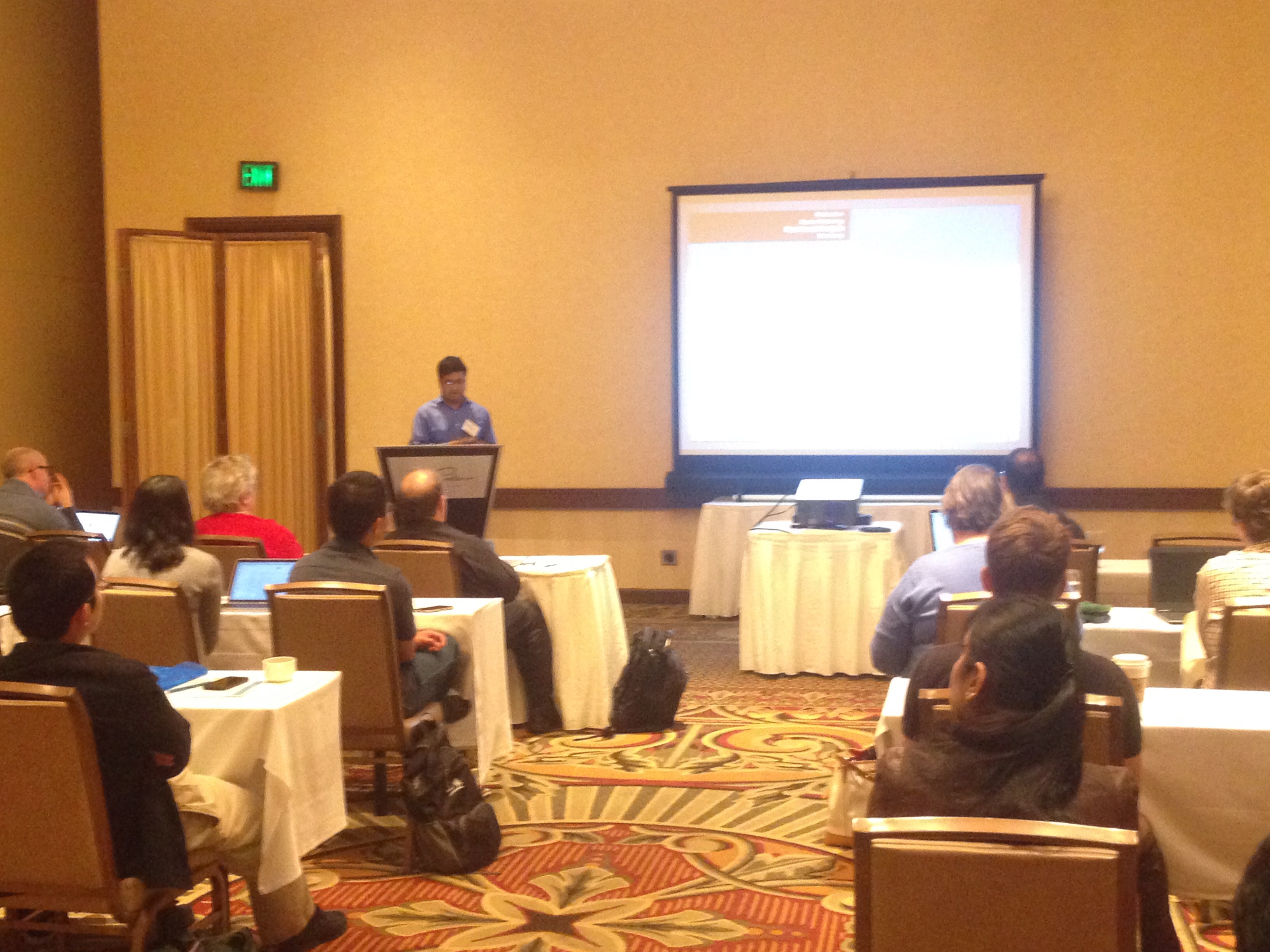
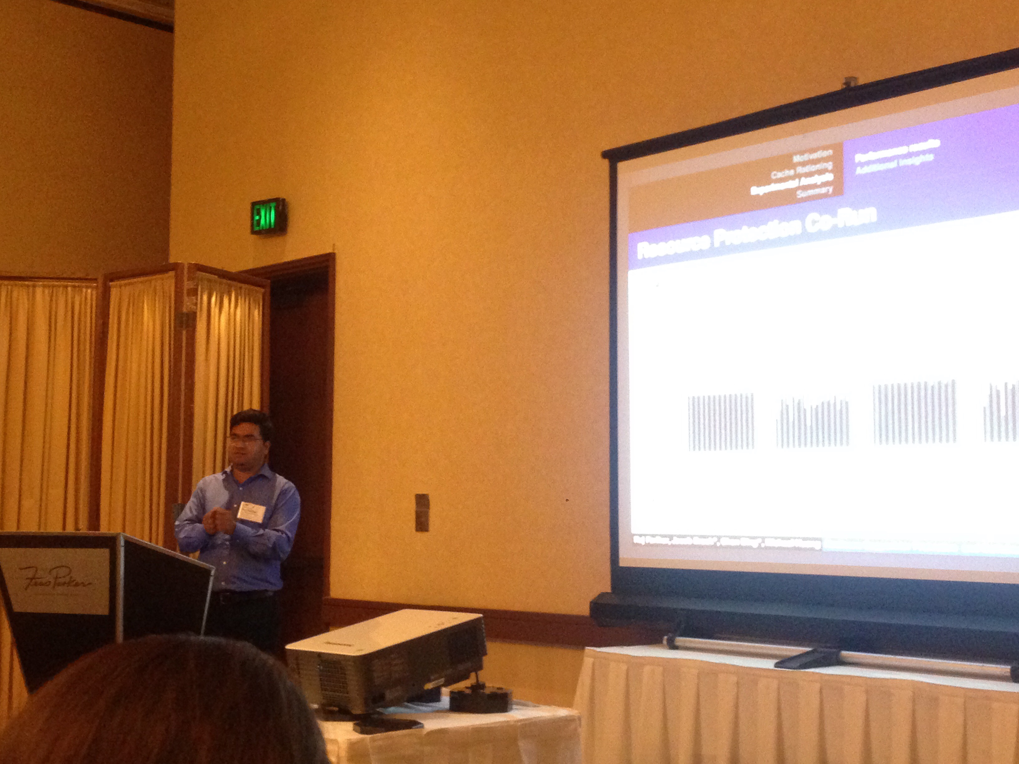
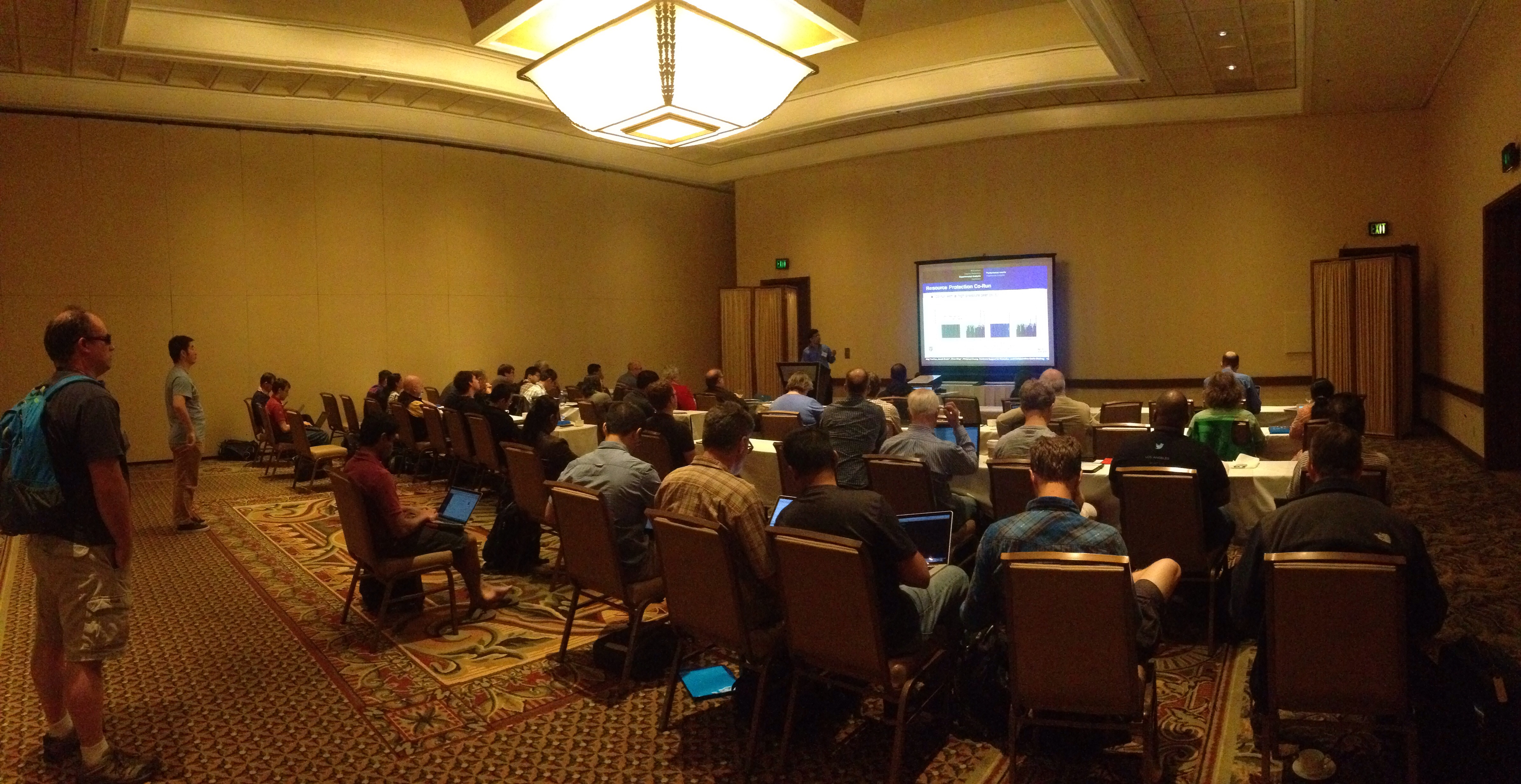
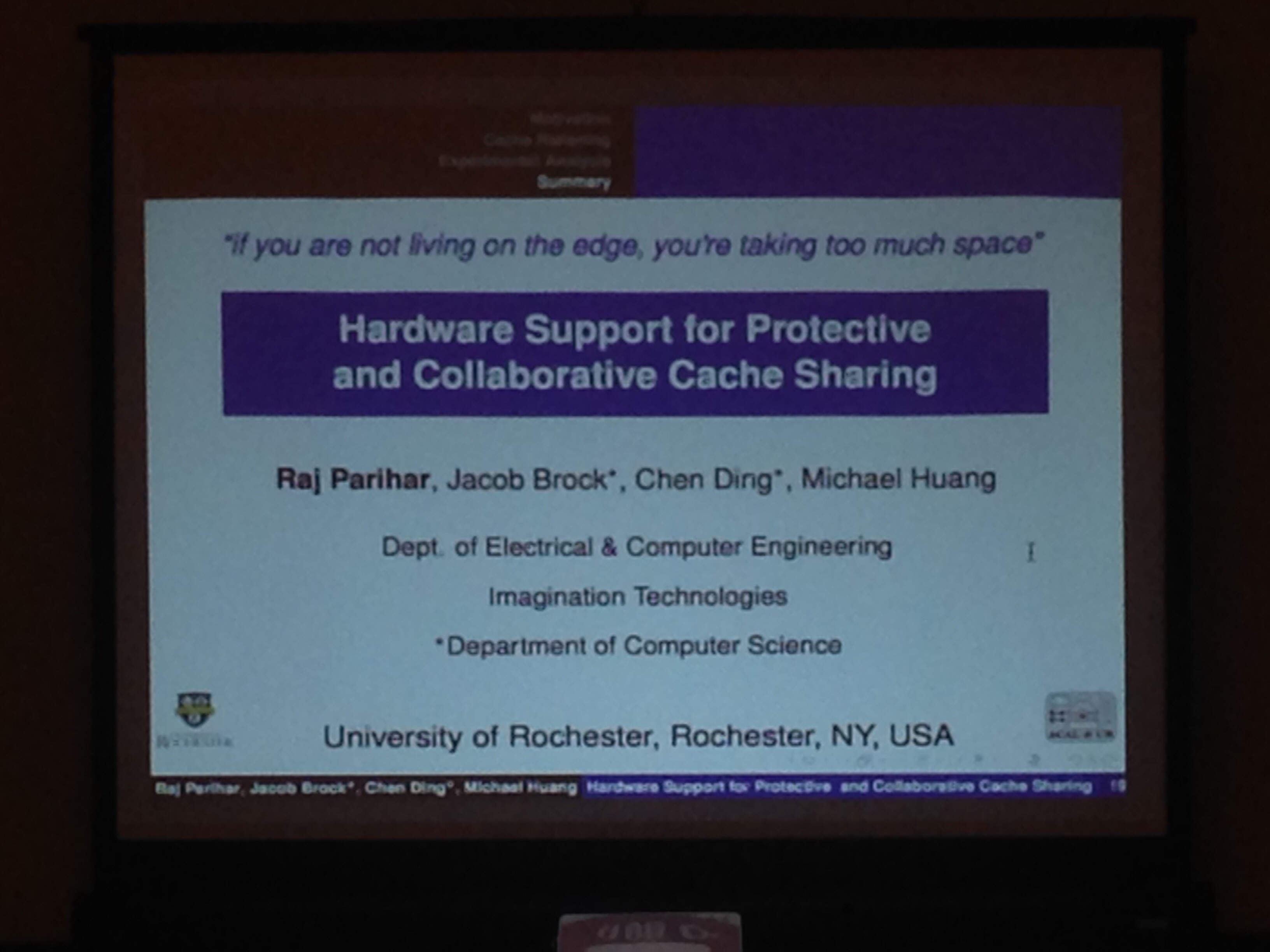
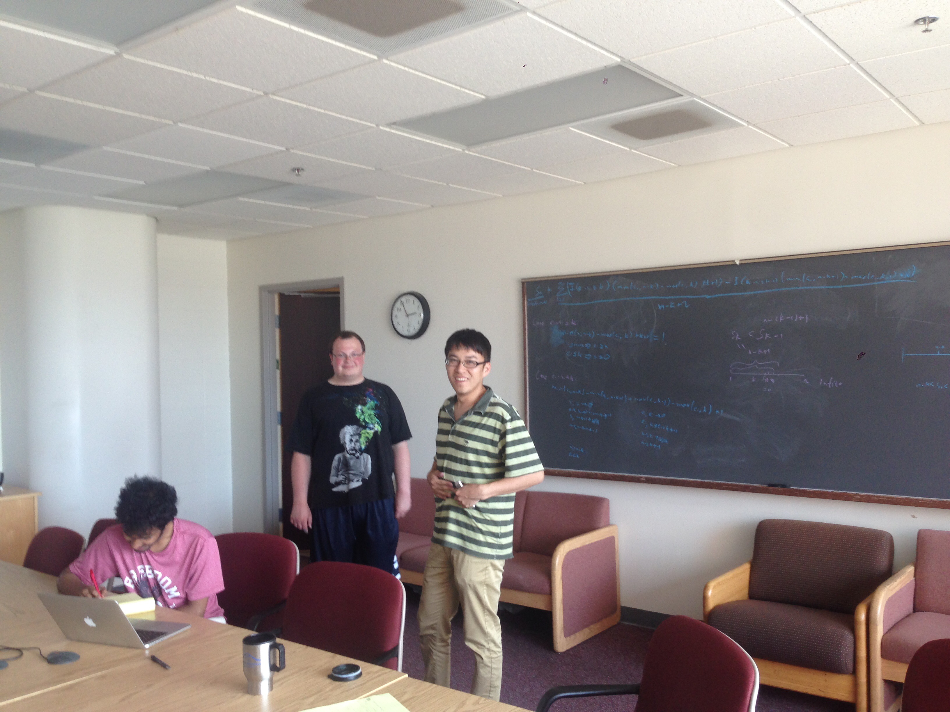
Photo 1: Friday before Memorial Day weekend, group work on proving the concavity property, after lunch under the sun at Sinbad.
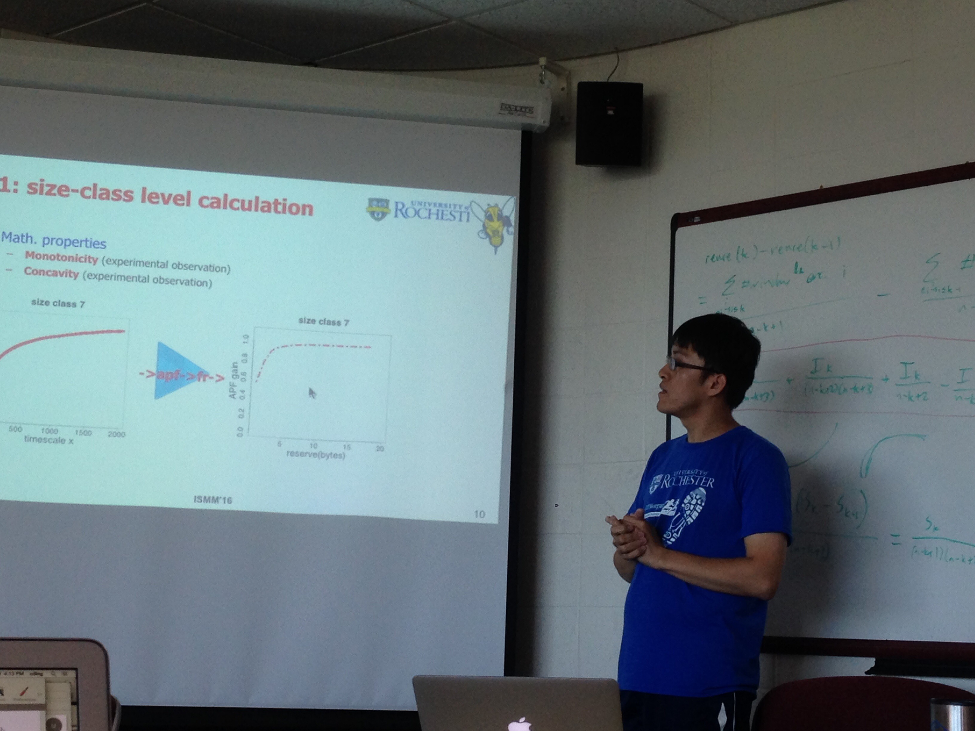
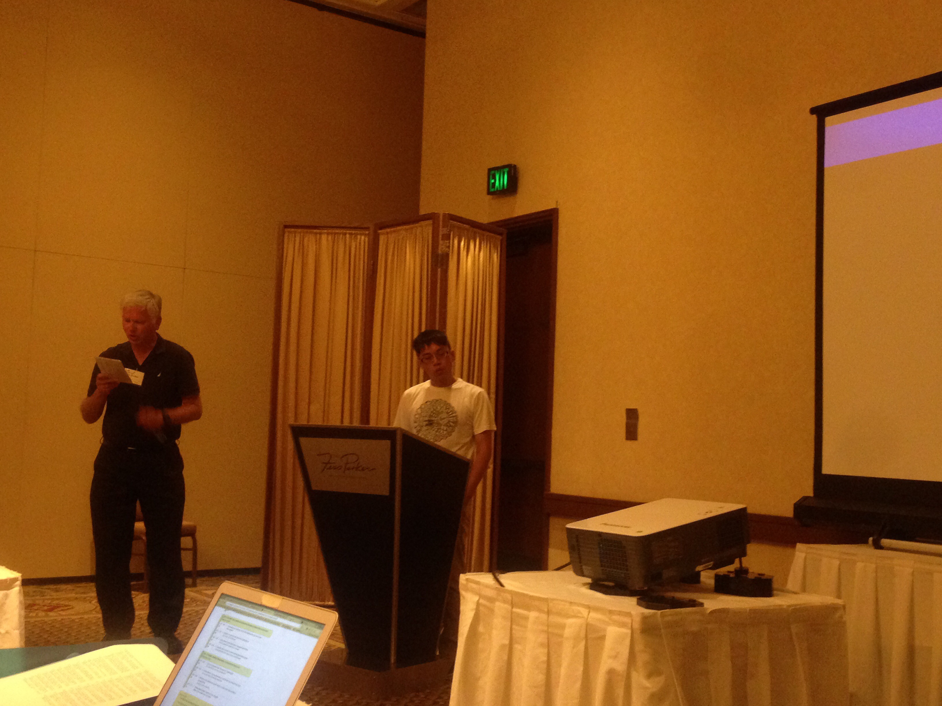
Photo 2: Thursday before ISMM, Pengcheng’s practice, helped by many comments/ questions/ suggestions from Michael, Sandya, Hao, and John and the presence of Ethan, Jie, Tianqin and Lizy.
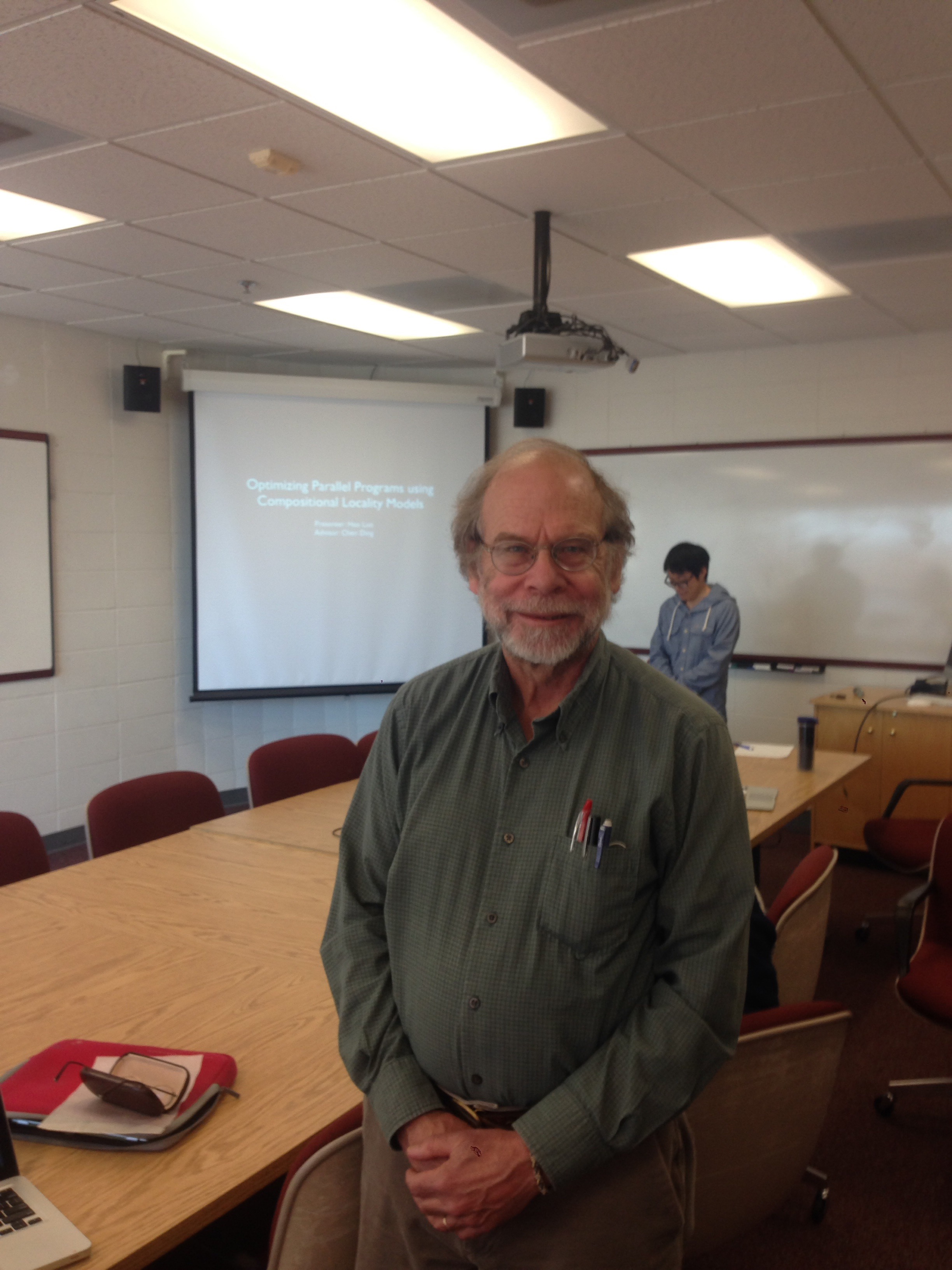
Photo 3: introduction by Hans-Boehm
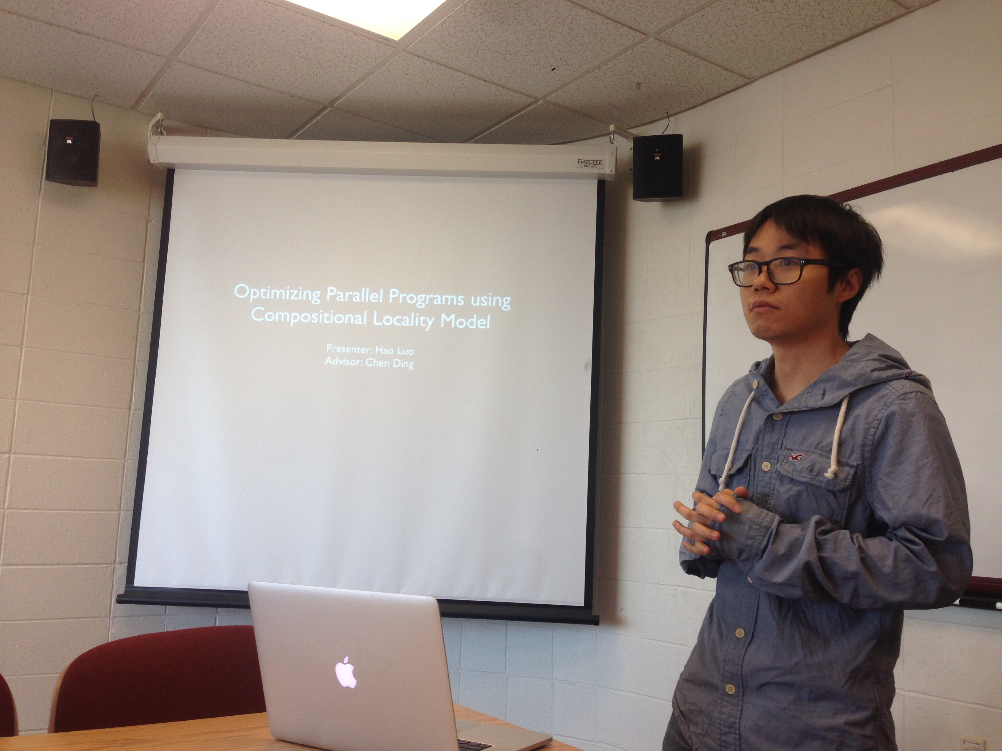
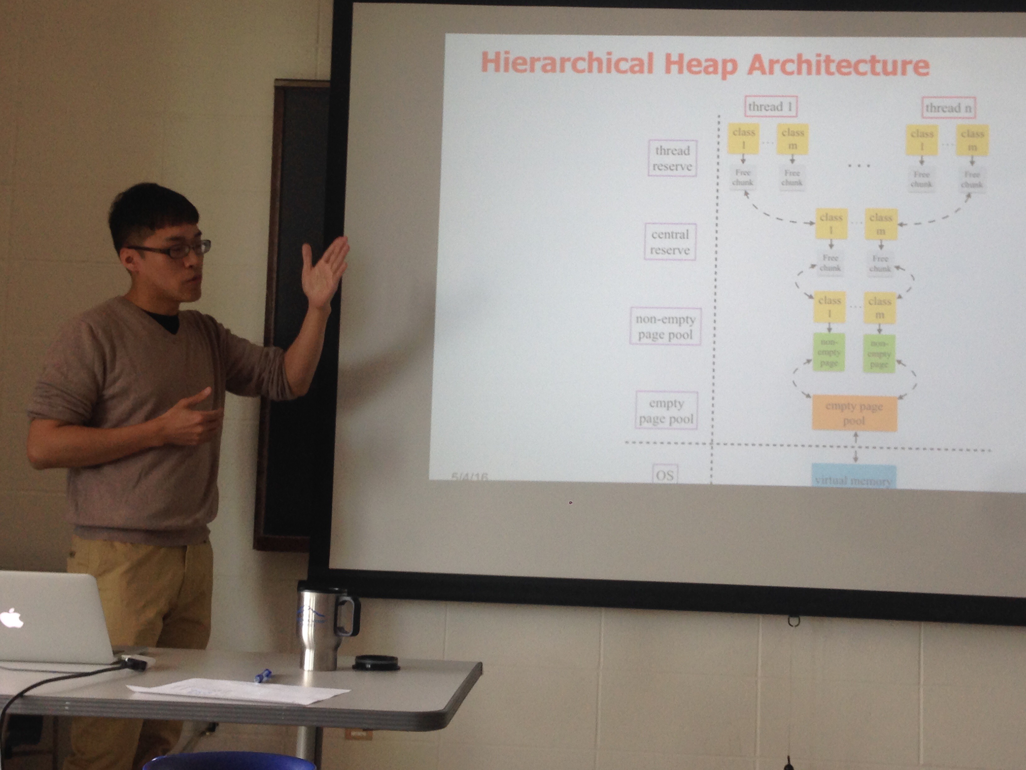
Hao: composable locality in parallel code – theory and optimization
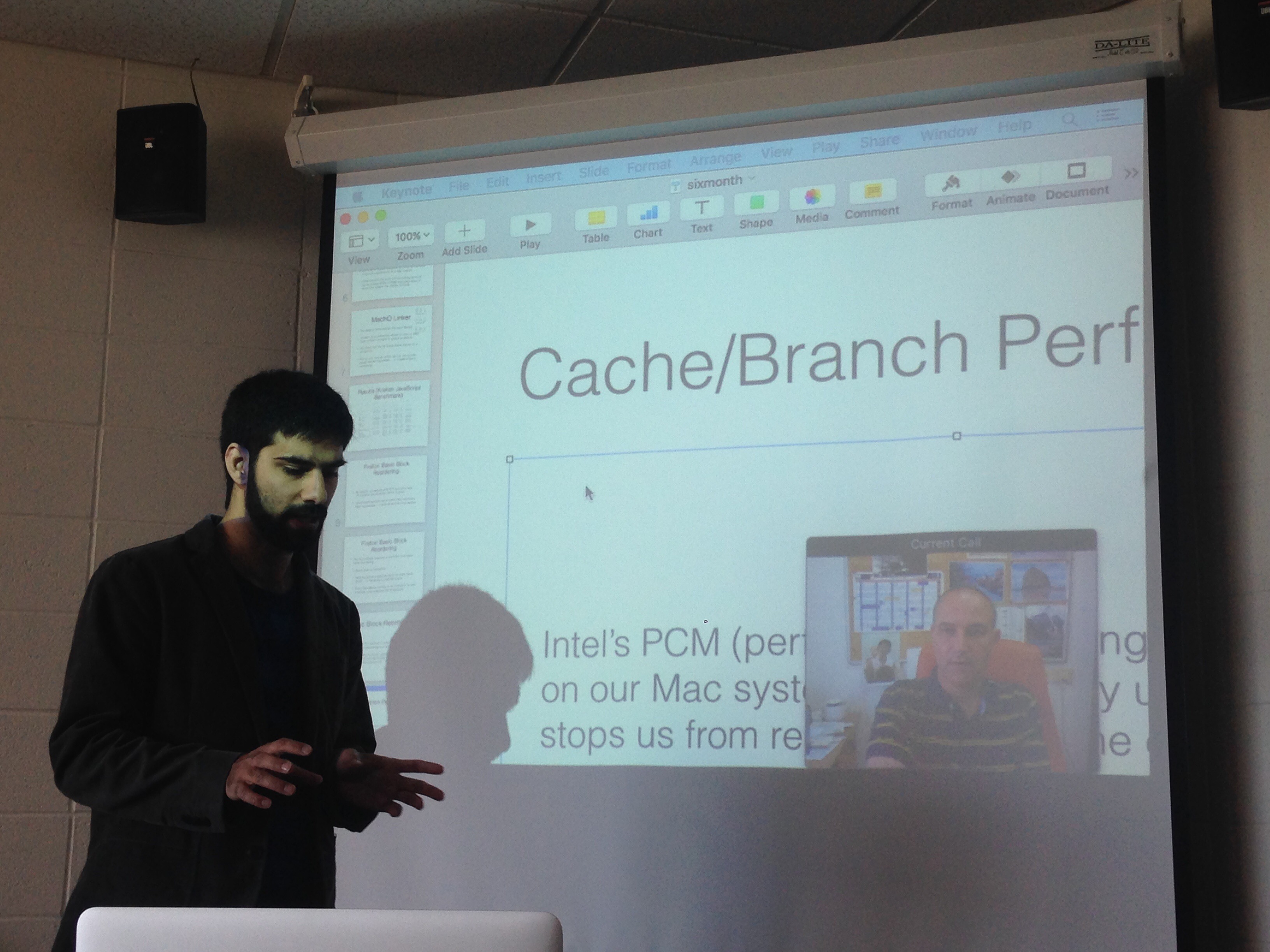
Rahman: optimizing code layout for very large software
Pengcheng: a higher order theory of memory demand
Jake: hybrid memory system management
Mike the award-winning thesis committee member
3rd spring Hackathon, 120 students, 36 hours, 17 projects, CS and data science.
Award winners: http://dandyhacks2016.devpost.com/
Many other good projects and presentations (ones I wrote down): Control-f books. Droplet. Electric go cart. Improvs. Vote2eat. Trump tweets. Medbook.tech. Musically.me. Naptimes. Serial port game. Pass the paragraph. Refugestudent.com. Trump bot. Rhythm fighter. Alg is simple. 3D gesture drawing. Virtual Tetris.


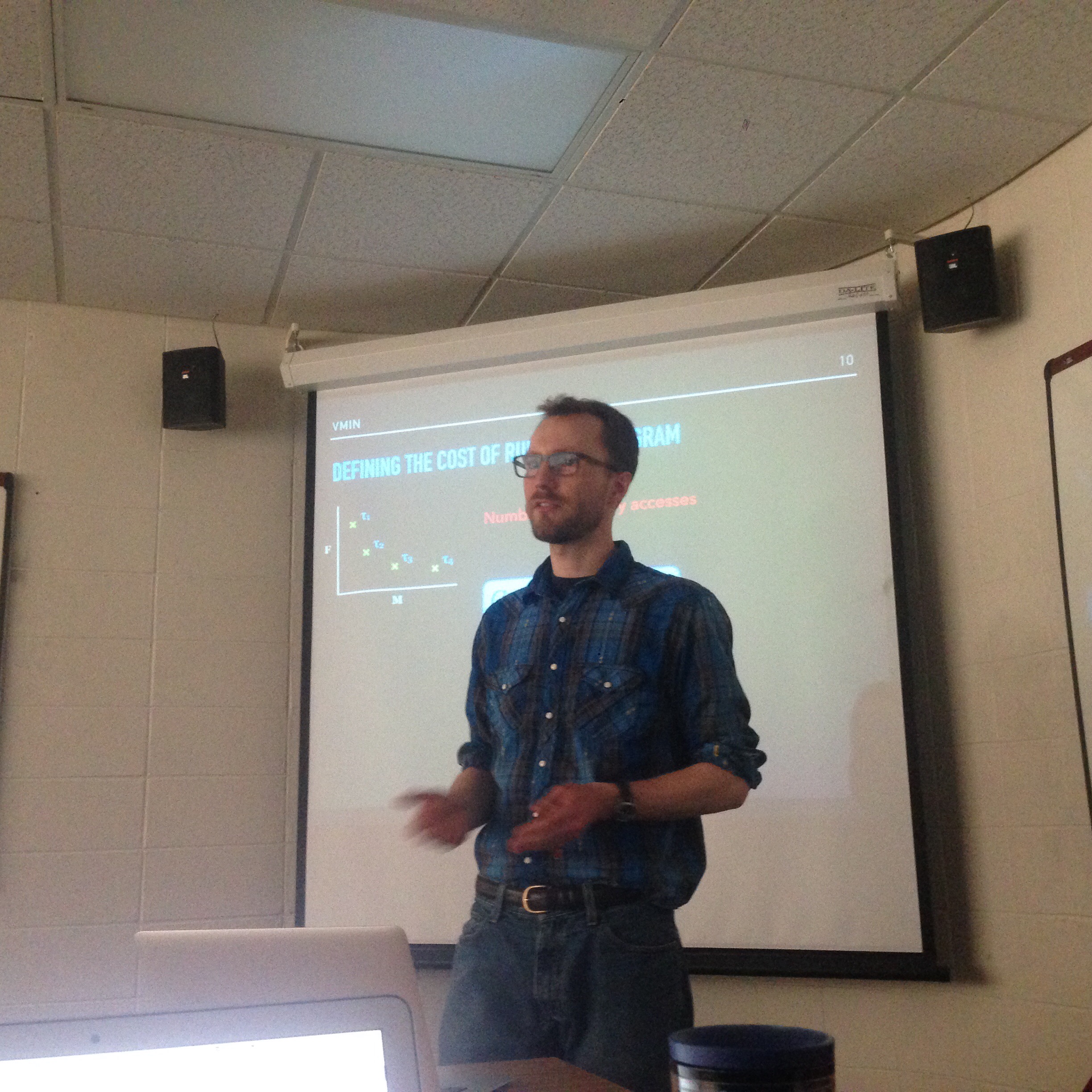
In their 1976 paper “VMIN — An Optimal Variable-Space Page Replacement Algorithm”, Prieve and Fabry outline a policy to minimize the fault rate of a program at any given amount of average memory usage (averaged over memory accesses, not real time). VMIN defines the cost of running a program as C = nFR + nMU, where n is the number of memory accesses, F is the page fault rate (faults per access), R is the cost per fault, M is the average number of pages in memory at a memory access, and U is the cost of keeping a page in memory for the time between two memory accesses. VMIN minimizes the total cost of running the program by minimizing the contribution of each item: Between accesses to the same page, t memory accesses apart, VMIN keeps the page in memory if the cost to do so (Ut) is less than the cost of missing that page on the second access (R). In other words, at each time, the cache contains every previously used item whose next use is less than τ = R accesses in the future. Since there is only one memory access per time step, it follows U that the number of items in cache will never exceed τ. Since this policy minimizes C, it holds that for whatever value of M results, F is minimized. M can be tuned by changing the value of τ.
Denning’s working set policy (WS) is similar. The working set W (t, τ ), at memory access t, is the set of pages touched in the last τ memory accesses. At each access, the cache contains every item whose last use is less than τ accesses in the past. As in the VMIN policy, the cache size can never exceed τ. WS uses past information in the same way that VMIN uses future information. As with VMIN, the average memory usage varies when τ does.
Compared with DRAM, phase change memory (PCM) can provides higher capacity, persistence, and significantly lower read and storage energy (all at the cost of higher read latency and lower write endurance). In order to take advantage of both technologies, several heterogeneous memory architectures, which incorporate both DRAM and PCM, have been proposed. One such proposal places the memories side-by-side in the memory hierarchy, and assigns each page to one of the memories. I propose that the VMIN algorithm described above can be modified to minimize total access latency for a given pair of average (DRAM, PCM) memory usage.
Using the following variables:
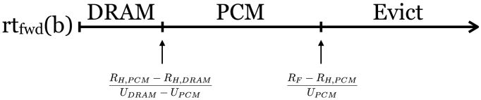
Define the cost of running a program as C = nFRF + nHDRAMRH,DRAM + nHPCMRH,PCM + nMDRAMUDRAM + nMPCMUPCM, where we are now counting the cost of a hit to each DRAM and PCM, since the hit latencies differ. If at each access we have the choice to store the datum in DRAM, PCM, or neither, until the next access to the same datum, the cost of each access b is rtfwd(b) * UDRAM + RH,DRAM if kept in DRAM until its next access, rtfwd(b) * UPCM + RH,PCM if kept in PCM until its next access, and RF if it is not kept in memory. At each access, the memory controller should make the decision with the minimal cost.
Of course, by minimizing the cost associated with every access, we minimize the total cost of running the program. The hit and miss costs are determined by the architecture, while the hit and miss ratios, and the DRAM and PCM memory usages are determined by the rents (UDRAM and UPCM, respectively). The only tunable parameters then are the rents, which determine the memory usage for each DRAM and PCM. The following figure (which assumes that UDRAM is sufficiently larger than UPCM) illustrates the decision, based on rtfwd(b):
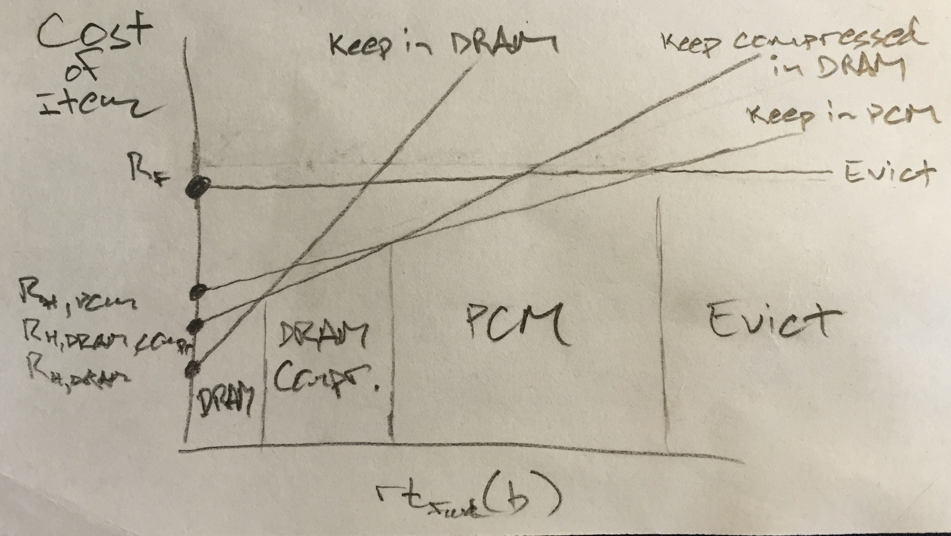
Update: an alternative diagram, showing the cost of keeping an item in each type of memory vs. the forward reuse distance (now including compressed DRAM):
Since the only free parameters are UDRAM and UPCM, this is equivalent to having two separate values of τ, τDRAM and τPCM in the original VMIN policy. The WS policy can be adapted by simply choosing a WS parameter for each DRAM and PCM.
If DRAM compression is an option, we can quantify the cost of storing an item in compressed form as rtfwd(b) * UDRAM \ [compression_ratio] + RH,DRAM_compressed.
